Week 5 - Rayleigh Taylor Instability

OBJECTIVE

1. To investigate practical CFD models that have been based on the mathematical analysis of Rayleigh Taylor waves
2. How these mathematical models have been adapted for CFD calculations.
3. Perform the Rayleigh Taylor instability simulation for 2 different mesh sizes with the base mesh being 0.5 mm. Compare the results by showing the animations.
4. Why we don't use a steady-state solver for these types of simulations?
5. Run one more simulation with water and user-defined material(density = 400 kg/m³, viscosity = 0.001 kg/m-s) for refined mesh. 
6. Significance of Atwood Number. 

SCOPE

• Basic understanding of Flow Instability 
• Transient Analysis.
• How to simulate a Multi-phase Problem.
• How to remove the floating-point exception.

SOFTWARE USED

• ANSYS SPACE CLAIM:- To design the fluid flow problem
• ANSYS MESHING:- Generation of mesh.
• ANSYS FLUENT:- To set up the physics; solution initialization and solving the fluid flow problems.

ABSTRACT

The Rayleigh–Taylor (R–T) instability occurs when a high-density (r1) fluid is placed over a lower-density (r2) fluid in a gravitational field. When the density interface is disturbed away from horizontal, the hydrostatic pressure acts to drive the heavier fluid into the lighter one, with the disturbance amplitude initially growing exponentially, but shortly afterward saturating and forming a characteristic mushroom shape, at least for some time. The creation of lengthy falling spikes interspersed with rising bubbles may be seen in the two-dimensional history of an initially sinusoidal perturbation at the fluid surface, with the heavier fluid on top.

DIFFERENT TYPES OF INSTABILITIES

The Kelvin Helmholtz Instability (KHI) is an application of hydrodynamic stability that can be seen in nature. It occurs when there are two fluids flowing at different velocities. The difference in the velocity of the fluids causes a shear velocity. at the interface of the two layers. The shear velocity of one fluid moving induces shear stress on the other which, if greater than the restraining surface tension, then results in instability along with the interface between them. This motion causes the appearance of a series of overturning ocean waves, a characteristic of the Kelvin–Helmholtz instability. Indeed, the apparent ocean wave-like nature is an example of vortex formation, which is formed when a fluid is rotating about some axis and is often associated with this phenomenon.

We can extend our understanding of the Rayleigh-Taylor instability to that of the Richtmyer-Meshkov instability (RMI). The pressure term does not necessarily need to be constant as-is for gravity, it can be impulsive as well. That is the case of the Richtmyer–Meshkov instability. In an instant, a large amount of vorticity gets deposited on the interface and the instability grows. The progression of the instability follows the progression of the constant acceleration case.

MATHEMATICAL ANALYSIS OF RAYLEIGH TAYLOR WAVES

1. K-L turbulence model for the self-similar growth of the Rayleigh-Taylor and Richtmyer-Meshkov instabilities

The turbulence model is developed to describe the self-similar growth of the Rayleigh-Taylor (RT) and Richtmyer-Meshkov (RM) instabilities. The model describes the dominant eddies in the mixing zone with evolutionary equations for their characteristic dimension and energy per unit mass. The equations are based on the successful buoyancy-drag models for RT and RM flows but constructed only with local parameters so that they can be applied to multidimensional flows with multiple shells of materials. The model has several unknown coefficients that are determined by comparing analytical and numerical solutions with RT and RM experiments.

2. Diesel Engine and KH RT model

The KH-RT (Kelvin-Helmholtz Rayleigh-Taylor) model is an enhanced version of the RD wave model. The KH-RT wave model comprises both Kelvin-Helmholz and Rayleigh-Taylor instabilities and it, therefore, has greater potential in providing enhanced simulation results. An interesting part of the KH-RT wave model is the KHinstability model which includes liquid viscosity as a
parameter, unlike the RD wave model. The objective of this study is to analyze the KH-RT wave atomization and drop breakup model and compare the predictive capabilities of wave models with respect to the experimental non-evaporating fuel spray of a large medium-speed diesel engine.

3. Wave Model

The WAVE breakup model was originally developed by Reitz and is based upon the temporal stability analysis of the Kelvin–Helmholtz instability for a liquid jet (density q1) with an inviscid outer gas phase (density q2). This Kelvin–Helmholtz instability causes ‘child’ droplets to be stripped from the liquid core of the jet, which is approximated by ‘parent’ droplets which have the same radius, R, as the injecting nozzle.

IMPORTANCE OF CFL NUMBER:

The Courant number can be used in Computational Fluid Dynamics (CFD) simulations to evaluate the time step requirements of a transient simulation for given mesh size and flow velocity and is linked to the Courant–Friedrichs–Lewy (CFL) stability condition of numerical schemes. The Courant–Friedrichs–Lewy or CFL condition is a condition for the stability of unstable numerical methods that model convection or wave phenomena.

GEOMETRIC DESCRIPTION 

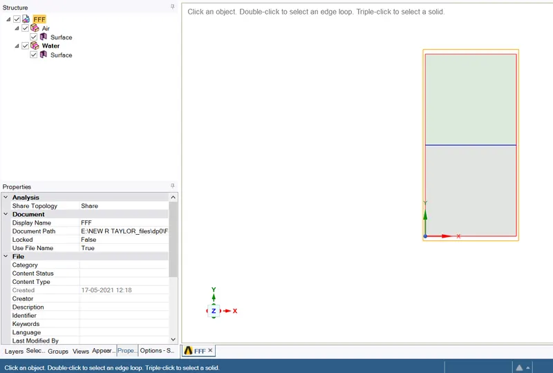
 For Two Dimensional Analysis, we use Ansys space claim to form our geometry by joining two flat sheets (square section each of side[ 20 mm * 20 mm])

SPACE CLAIM

water-side (top) [ 20 mm * 20 mm]

air-side (bottom)[ 20 mm * 20 mm]

Share Tapology ON

    

MESH 

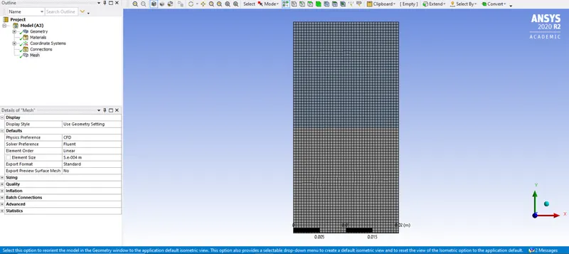
CASE 1:

ELEMENT SIZE : 0.5 mm

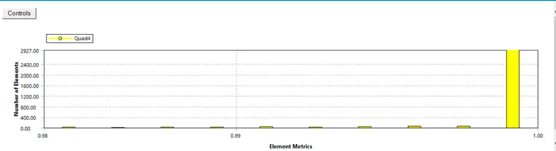
MESH QUALITY

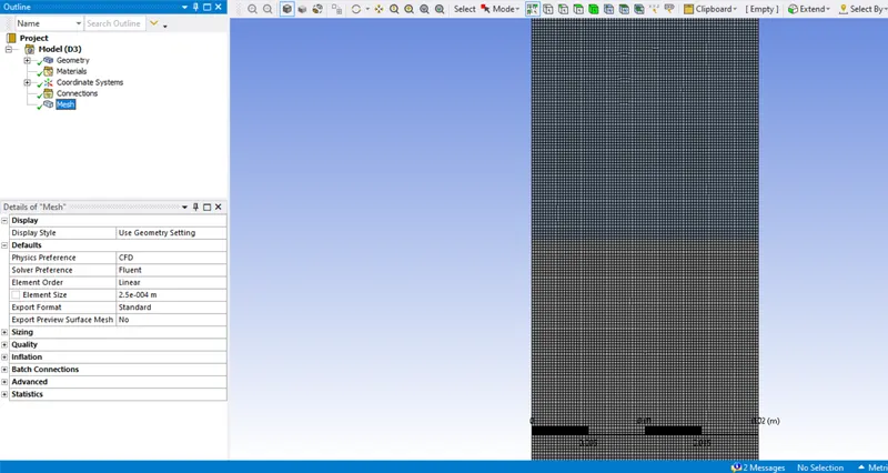
CASE 2 :

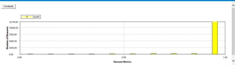
ELEMENT SIZE: 0.25 mm

MESH QUALITY:

CASE 3:

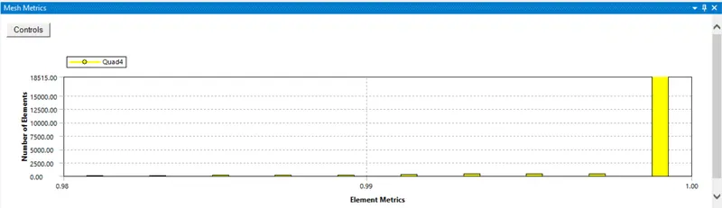
ELEMENT SIZE: 0.2 mm

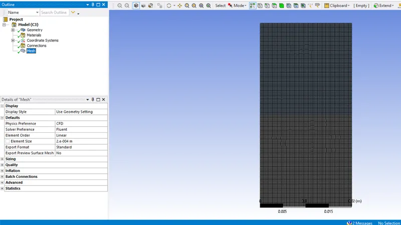
 MESH QUALITY:

FLUENT SOFTWARE:-

SOLVER: Transient - Pressure Based

Gravity : in y-direction [-9.81 m/s^2]

Flow Type: Laminar  

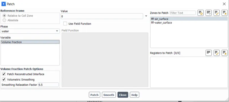
Model type: Multiphase Flow[ VOF method ]

Method: Implicit 

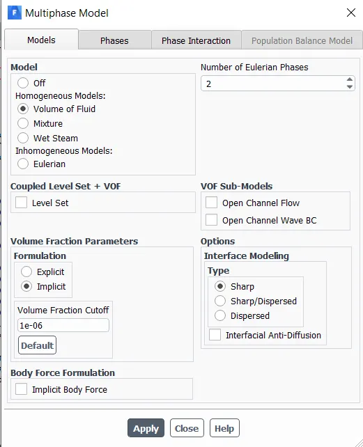
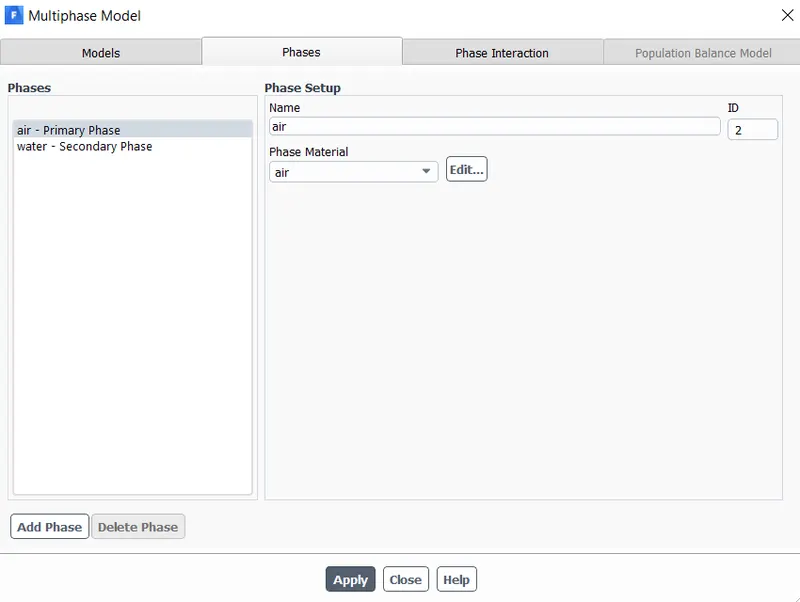
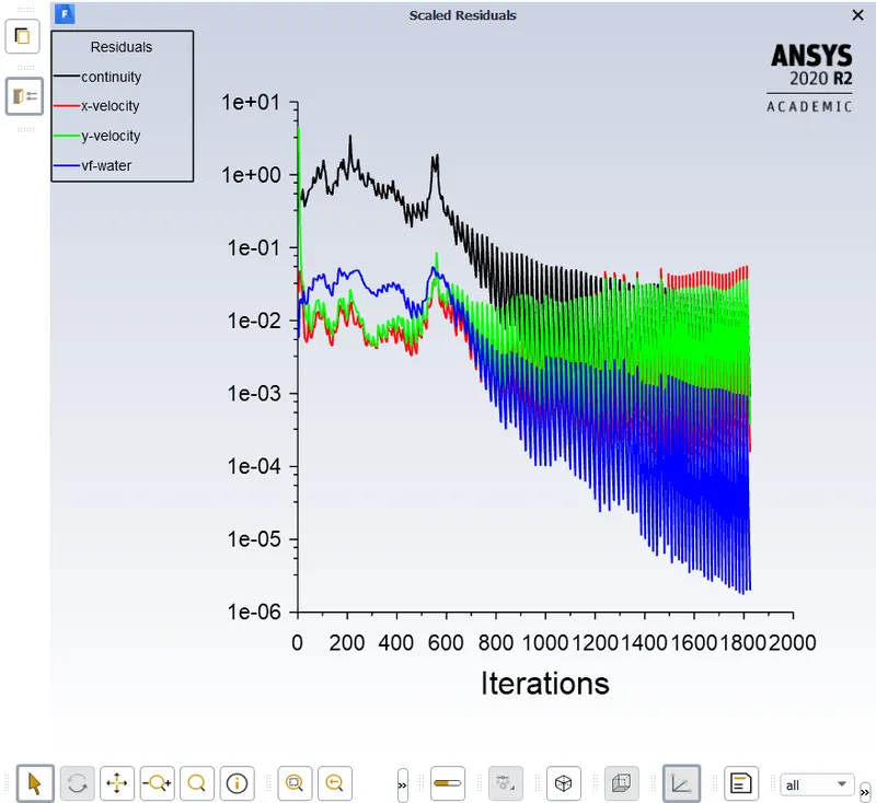
CASE 1: ELEMENT SIZE= 0.5 mm

time step = 0.005

CASE 2: ELEMENT SIZE= 0.25 mm

time step = 0.005

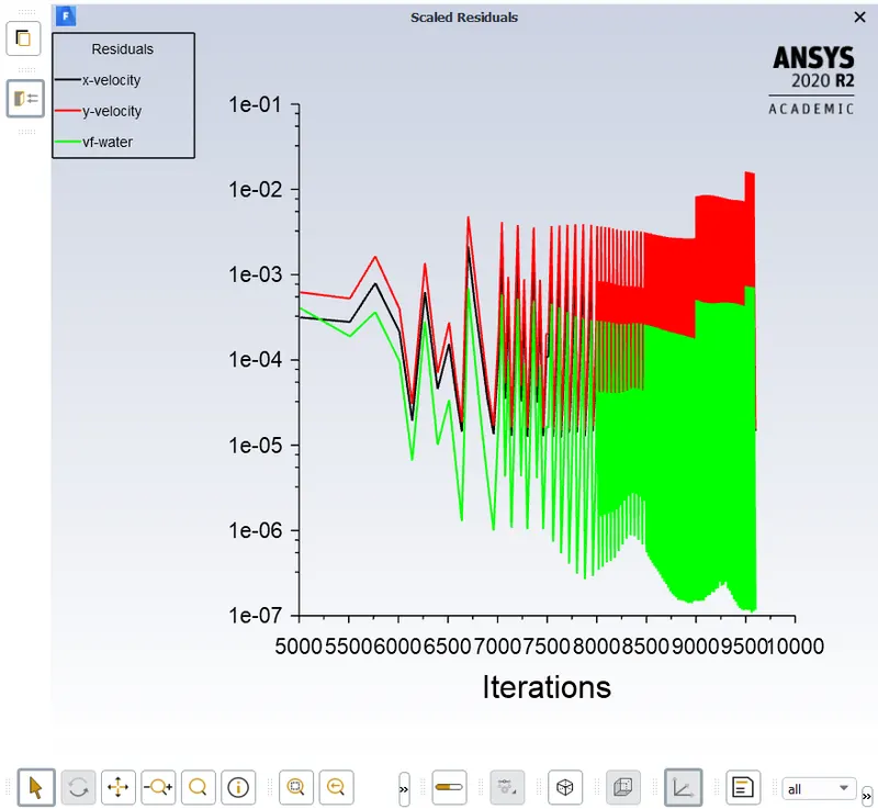
CASE 3 :ELEMENT SIZE= 0.2 mm

time step = 0.002

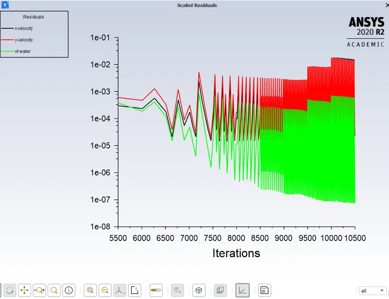
USER DEFINED MATERIAL:

ELEMENT SIZE= 0.2 mm

time step = 0.002

density = 400 kg/m³, viscosity = 0.001 kg/m-s

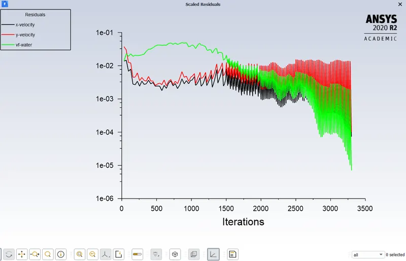
Why we don't use a steady-state solver for these types of simulations?

Comparison between steady and transient analysis

• This is the first and perhaps the biggest decision in CFD.
• Steady-state simulation computes the fully developed solution that does not change in time.
• When steady-state used the mean values are computed.
• The steady-state simulation is way faster than transient.
• Transient simulation computes the instantaneous values at each time for each quantity.
• Transient simulation has much higher requirements comparing to steady-state. 
• The results of transient simulation may be more comprehensive.

 

 Since we have to get the instability pattern at the interface of two fluids which is time-dependent and steady-state solver is independent of time. We are not concerned about the final answer. we want to visualize at each and every instant. That's why we prefer transient state analysis of Rayleigh Taylor Instability.

Significance od Astwood Number at 

The Atwood number (A) is a dimensionless number in the fluid dynamic used in the study of hydrodynamic instabilities in density stratified flows. It is a dimensionless density ratio defined as

Where

 = density of the heavier fluid.

 = density of the lighter fluid.

FOR AIR -WATER 

 = 998.2 kg/m^3.   = 1.225 kg/m^3

`A= (998.2-1.225)/(998.2+1.225)`

  A = 0.998

FOR WATER -USER DEFINED 

 = 998.2 kg/m^3.   = 400 kg/m^3

         `A= (998.2-400)/(998.2+400)`

          A = 0.428

Smaller Atwood numbers result in longer delay distances. Higher Atwood numbers shorten the delay and its associated distance, providing a longer development period for the R–T mixing. In Rayleigh–Taylor instability, the penetration distance of heavy fluid bubbles into the lighter fluid is a function of the acceleration time scale.

MORE REFINED MESH, HEAVIER FLUID TAKE MORE TIME TO SETTLE BETTER FLOW VISUALISATION. HOWEVER, TIME CONSUMING.

References

[1] Fluid dynamic instabilities: theory and application to the pattern forming in complex media.

[4] https://www.cfdsupport.com/OpenFOAM-Training-by-CFD-Support/node356.html

[5] K-L turbulence model for the self-similar growth of the Rayleigh-Taylor and Richtmyer-Meshkov instabilities

[6] DYNAMICAL METEOROLOGY | Kelvin–Helmholtz Instability