Week 5 - Rayleigh Taylor Instability

Rayleigh Taylor Instability

AIM:

1. Perform the Rayleigh Taylor instability simulation for 2 different mesh sizes with the base mesh being 0.5 mm. Compare the results by showing the animations( Attach them from your google drive). Observe the differences in the animation and explain the effect of mesh size on simulation. Also, explain why a steady-state approach might not be suitable for these types of simulations.[ Choose Air and Water for this simulation]
2. Run one more simulation with water and user-defined material(density = 400 kg/m³, viscosity = 0.001 kg/m-s) for refined mesh.

INTRODUCTION:

The purpose of this problem is to simulate a two-dimensional Rayleigh-Taylor instability problem using the classical method of Finite Element analysis of a multiphase model using ANSYS FLUENT. The governing equations consist of a system of coupled nonlinear partial differential equations for conservation of mass, momentum, and phase transport equations. The study focuses on the transient state simulation of Rayleigh Taylor waves and subsequent turbulent mixing in the two phases incorporated in the model. The Rayleigh Taylor instability is the instability of an interface between two fluids of different densities which occurs when the lighter fluid is pushing the heavier fluid in a gravitational field. The problem was governed by the Navier-Stokes and Cahn-Hilliard equations in a primitive variable formulation. The Cahn- Hilliard equations were used to capture the interface between two fluids systems.

Q: What are some practical CFD models that have been based on the mathematical analysis of Rayleigh Taylor waves? In your own words, explain how these mathematical models have been adapted for CFD calculations.

A:

Kevin-Helmholtz Instability:

The Kelvin–Helmholtz instability typically occurs when there is velocity shear in a single continuous fluid, or additionally where there is a velocity difference across the interface between two fluids. A common example is seen with the wind blowing over water, the instability constant is able to manifest itself through waves on a water surface. The Kelvin-Helmholtz instability is not only restricted to a water surface as clouds, but is evident through other natural phenomena as the ocean, Saturn's bands, Jupiter's Red Spot, and the sun's corona.

In the case of a short wavelength, if surface tension is ignored, two fluids in parallel motion with different velocities and densities yield an interface that is unstable for all speeds. However, surface tension is able to stabilize the short-wavelength instability and predict stability until a velocity threshold is reached. The linear stability theory, with surface tension, included, broadly predicts the onset of a wave formation as well as the transition to turbulence in the important case of wind over water.

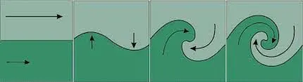
In the case of a short wavelength, if surface tension is ignored, two fluids in parallel motion with different velocities and densities yield an interface that is unstable for all speeds. However, surface tension is able to stabilize the short-wavelength instability and predict stability until a velocity threshold is reached. The linear stability theory, with surface tension, included, broadly predicts the onset of a wave formation as well as the transition to turbulence in the important case of wind over water.

It was recently discovered that the fluid equations governing the linear dynamics of the system admit a parity-time symmetry, and the Kelvin-Helmholtz instability occurs when and only when the parity-time symmetry breaks spontaneously.

Plateau-Rayleigh Instability:

The Plateau–Rayleigh instability, often just called the Rayleigh instability, explains why and how a falling stream of fluid breaks up into smaller packets with the same volume but less surface area. It is related to the RTI and is part of a greater branch of fluid dynamics concerned with fluid thread breakup. This fluid instability is exploited in the design of a particular type of inkjet technology whereby a jet of liquid is perturbed into a steady stream of droplets.

The driving force of the Plateau–Rayleigh instability is that liquids, by virtue of their surface tensions, tend to minimize their surface area. A considerable amount of work has been done recently on the final pinching profile by attacking it with self-similar solutions.

The following figure shows the diagram for Plateau-Rayleigh instability:

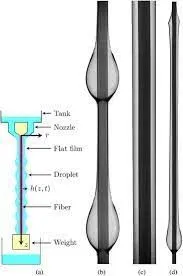
The flow begins with tiny perturbations in the stream. Some grow and some decay over time. The growth of some may be faster and that of others might be slower. The growth rate of the perturbations can be mapped as a function of the wavenumber and radius of the cylindrical system. Assuming initially that all component amplitudes are roughly equal, the wavenumbers are checked. As time progresses the component with maximum growth rate will be the one that pinches the stream into drops. Young’s Laplace equation uses the concept of Cylinder radius and Radius of Curvature (ROC) to assess the pressure applied to the stream. As the cylinder radius decreases (at the trough), pressure due to surface tension increases, and as the Radius of Curvature is negative at the trough, the pressure decreases. This might lead to a small cancellation of the pressure effects due to both phenomenons.

Geometry

Preparation of geometry

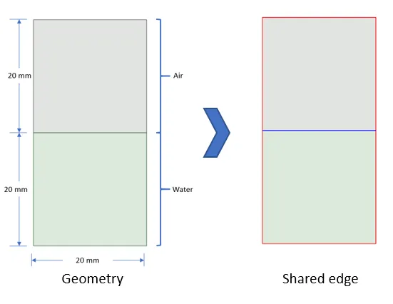
The geometry is essentially two squares, one on top of another side 20 mm. The top square has been named 'water' and the bottom square 'air'. The common edge between the domains was shared using the share tool in Workbench. 2 D geometry has been created in Spaceclaim. The air and water domain are created of size 20mm x 20 mm respectively as shown in fig. Share topology has been used to share the domain. The blue edge is the shared edge between the air and water domain.

Meshing

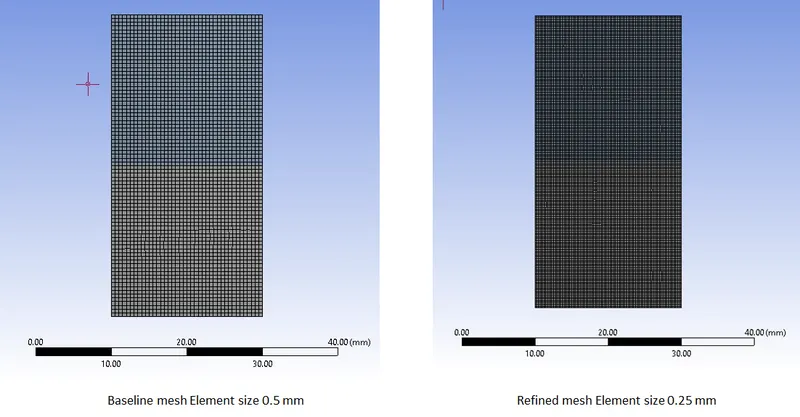
The refined mesh is created for an element size of 0.25mm. Basic Meshing is used. To improve the details Inflation layers can be added at the boundaries.

SETUP:

Since the problem statement is considered for a low Mach number, a Pressure Based Solver is considered for the simulation. The Laminar model was used for the respective test case calculations. A Transient State simulation is run. The Multiphase option is selected and the Volume of Fluids Solving method is employed. The respective Materials were copied from the Fluent Database and the phases were input with the materials. Standard Initialization is used for t=0 and 500 iterations were run for each case. Each phase was patched with a volume fraction of water (1 for water and 0 for air/user material). After Standard Initialization, to patch both the domains to the respective materials, provided a volume-fraction value of 1 to water and 0 to air and user-defined material.

Results

Baseline Meshing with element size 0.5 mm

Refined mesh with element size 0.25 mm

Refined mesh with element size 0.25 mm ( User-defined Material and water mixture)

Finer mesh captures the instability better than the coarse mesh, but it takes more time for the heavier fluid to settle down. So it is computationally expensive but produces results with better accuracy.

Since the simulation involves capturing instabilities that are changing in an unpredictable manner as a function of time, the transient approach is preferred over the steady-state approach.

CONCLUSION:

1. For the first test case, a bubble plum was observed. When the mesh was refined, some changes in the flow created a smoother plot over time.
2. For the user input material, where the Atwood number is reduced, the flow progressed with symmetric finger-like protrusions and took a larger time to stabilize.
3. The Transient State analysis was used to capture the fluctuations in the instability at every time step.
4. In the first two cases, for higher Atwood numbers the bubble-like protrusions were uniform and significant in the refined case. Most of the denser fluid traversed along the wall because of the bubble plumes.
5. A more unstable mixing was observed for the third case at a lower Atwood number. The multiple protrusions led to better mixing of fluids in this case.
6. Due to the lower density difference between the user-defined material and water, the instability was observed at a later time step, and the mixing and stabilizing of the fluids took a longer time.