Week 4 - CHT Analysis on Exhaust port

Aim

To determine the coefficient of convective heat transfer as well as temperature variation with respect to velocity in accordance with conservation of mass phenomenon,

Introduction

The exhaust manifold is the key component in a 4- stroke IC engine. The exhaust manifold is mounted on the cylinder head of an engine. The exhaust manifold collects exhaust gases from multiple cylinders into one pipe. At the exhaust stroke, the exhaust valve opens and the inlet valve remains closed that time piston starts moving from bottom dead centre to top dead centre sweeps out the burnt gases from the cylinders

Conjugate Heat Transfer Analysis

It represents a class of multi-physics problems where fluid flow affects the thermal behaviour of the structure, which in turn affects the fluid flow. For conjugate heat transfer analyses, the solid material conduction and the fluid convection are analysed simultaneously. The conductive heat transfer in a solid region is coupled to the convective heat transfer in a neighbouring fluid flow. The Conjugate Heat Transfer (CHT) analysis type allows for the simulation of heat transfer between solid and fluid domains by exchanging thermal energy at the interfaces between them. Typical applications of this analysis type exist as, but are not limited to, the simulation of heat exchangers, cooling of electronic equipment, and general-purpose cooling and heating systems.

Conjugate Heat Transfer Analysis of Exhaust Manifold

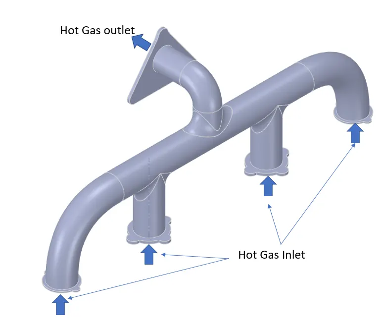
1) Geometry

2) Fluid domain

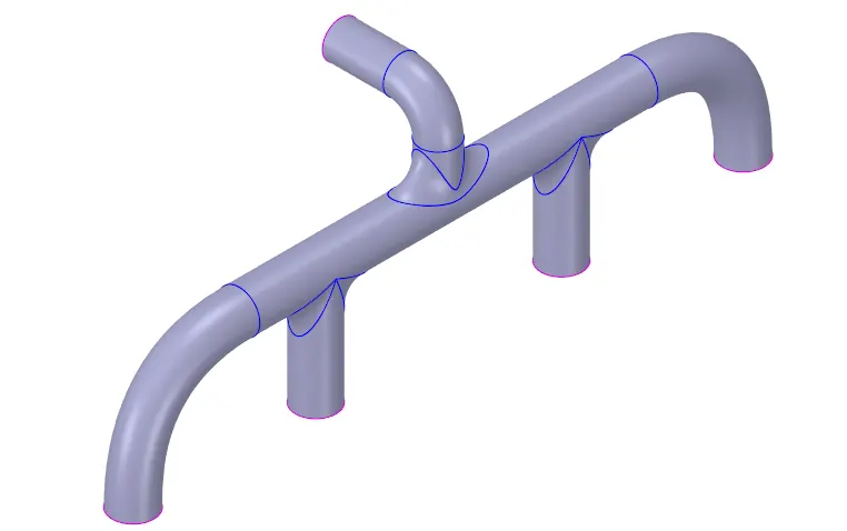
The fluid domain has been created in the SpaceClaim tool after geometry cleanup. As this analysis include Conjugate heat transfer, in order to get the conformal mesh, share topology to be assigned. The pink edges in the below diagram show share surfaces.

3) Meshing

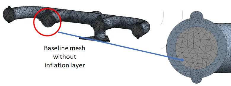
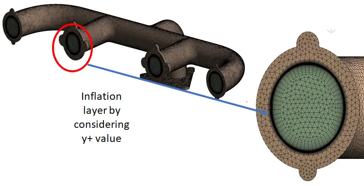
Name selection :

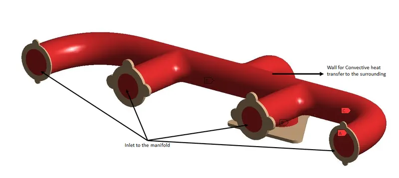
Case I Baseline mesh

Number of elements : 24523

Case II Refined mesh

Number of elements :49823

4) Case setup

Solver time = Steady state

Solver type = Pressure Based

Turbulence model = k-epsilon

Solid material = aluminium

fluid material = air

Boundary condition

Velocity at inlet = 5 m/s

Temperature at inlet = 700k

Heat transfer coefficient at the outer wall = 20 W/m^2-k (Outer convective wall)

5) Results

Case I : Basline mesh

Contour plotes at section plane

Contour plotes on convetive wall

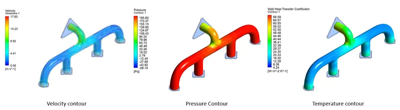
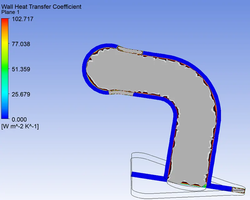
It can be observed a highly irregular heat transfer coefficient plot, that is due to the baseline mesh, any how since the there is a high temperature fluid going through this portion with a high velocity, the reddness of the plot which shows heat is being transferred at hight rate in nearly the entire section.

Case II : With inflation layer

Contour plots at section plane

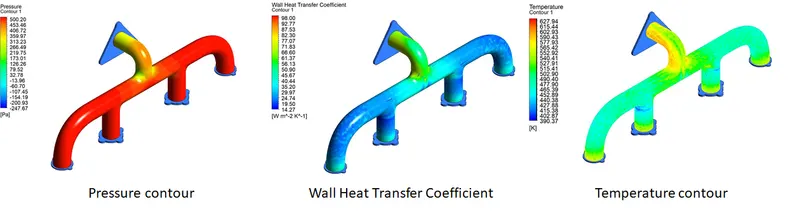
These plots are much finer and smoother looking visuals and it can see the velocity variations in the outlet port zone much clearly. The first mesh plot gave slightly different velocity variations than this one. The maximum velocity at the curve section in red color is more than from the Baseline mesh.

The velocity, created in a plane in between the exhause manifold, we can see how the velocity is less at the beginning and quickly escalates by almost 10 m/s when it enters the outlet port. This occurs due to mass conservation, hence when more mass of fluid is accumulated, and since its directily proportional to velocity in momentum equation, there is increase of velocity.

The temperature at inlet being 700k. It can be observe that it has most highest temperature, but as the fluid is moving it's slightly reducing in temperature at some sections.

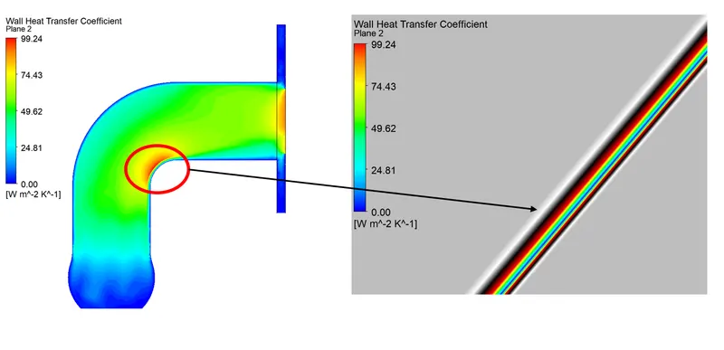
Contour plots on convective wall

Wall heat transfer coefficient with a velocity contour plot

3. Validation of the HTC prediction from the simulation:-

The overall heat transfer rate for combined modes is usually expressed in terms of heat transfer coefficient. The general definition of the heat transfer coefficient is

Where,

h = heat transfer coefficient (W/m^2-k)

q = heat flux (W/m^2)

dt = temperature difference between the solid surface and surrounding fluid area (K)

The heat transfer coefficient obtained from the simulation can be verified by conducting experiments but the experimental assessment of the heat transfer coefficient gets complex especially when calculation the small fluxes.

The heat transfer coefficient is often calculated from the nusselt number,

Where,

Nu = nusselt number (dimensionless number)

h = heat transfer coefficient (W/m^2-k)

k = thermal conductivity (W/m-k)

Since the mode of heat transfer is forced convection in internal flow the nusselt number can be calculated from the below equations,

For internal flow, laminar flow,

• Seider and tate give the following correlation for the entrance effects in laminar flow in tubes,

where,

Re = Reynolds number

Pr = Prandtl number

D = Inner diameter

L = Characteristic length

Mu(b) = Fluid viscosity at bulk mean temperature

Mu(w) = Viscosity at wall surface

For fully developed laminar flow the nussselt number is constant and is equal to 0.36 and the fully developed flow and entrance is combined to form an equation given by mills,

For internal flow, turbulent flow,

Dittus Boelter correlation can be used for finding nusselt number when forced convection is the only mode of heat transfer and is given by the equation,

Where,

j = mass flux

d = hydraulic diameter

Mu = fluid viscosity

Cp = isobaric heat capacity

k = thermal conductivity

n = 0.4 for heating and 0.33 for cooling

4. Factores on which the accuracy of the prediction depend on:-

1. Refining the mesh by creating the inflation layers and increasing the number of elements which helps in obtaining more clear and accurate contours.
2. Setting up proper boundary conditions.
3. Selecting a proper turbulence model for solving the problem.

Conclusion :

1. From the above simulation it is clear the heat transfer coefficient is higher at the reagion where the velocity is higher. In case 1, the maximum heat transfer coefficient is 118.7 W/m^2-k and maximum velocity in outlet port is 30.78 m/s where as in case 2, the maximum heat transfer coefficient is 113 W/m^2-k and maximum velocity at the outlet port is 30.78 m/s.
2. The pressure is high at the inlet ports and decreases at the outlet port. The pressure near the inlet walls is 517.6 Pa and the pressure near the outlet walls is 336.9 Pa.
3. The contours appear more accurate and clear with the increase in number of elements and refining the mesh at the inner wall by creating the inflation layers. And also the value of the HTC changes after refining the mesh by creating inflation layers near the inner walls.