Week 5 - Mid term project - Solving the steady and unsteady 2D heat conduction problem

Solving the steady and unsteady 2D heat conduction proble

Title : Steady state heat conduction analysis using Jacobi, Guass-Seidel and Successive over relaxation iteration method

Abstract

This project is focuses on analysis of 2D heat conduction using point iterative techniques. This analysis is divided as steady state analysis and transient state analysis. Analysis has been done by using Jacobi, Guass-Siedel and SOR (Successive-over relaxation) iteration method. As a result of this analysis, number of iteration and required to converge the solution has been determined as well as time required to achieve steady state can helps to determine effective method for analysis. Equation has been solved at each node. The governing equation are descritized by using central differencing method of second order accuracy.

Problem statement :

The 2D geometry is subjected to different temperature at it's boundary. The change in temperature of the plate based on time and steady state condition of the plate has to be analyzed. The effect of implicit and explicit method for describing conduction equation is to be used.

Governing equation :

The conduction equation for 2D geometry is given by,

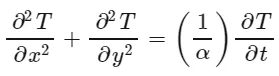.................Unsteady condition

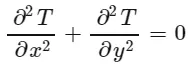...........................Steady state condition

Descritization :

Discritization of above equation is given by,

....along 'x' axis

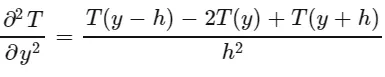....along 'y' axis

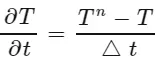............................Based on time

For the steady state condition, temperature is varies to achive steady state. Therefore variation of temperature at different grid point is given by,

Temperature variation at different grid point is given by,

This descritised equation is used for iterative method.

For transient condition, The conduction equation is given by,

While solving this equation using explicit method, temperature at next grid pint is deermined by based on adjecent grid point temperature. The stability of solution is depends on time step value. As time step increase, solution may get unsteable and leads to divergence of solution. The allowable time step can be given by,

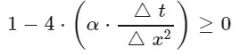
Therefore implicit method is used to avoid unstable condition during iteration.

Results :

Conclusion :

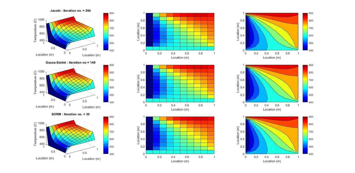
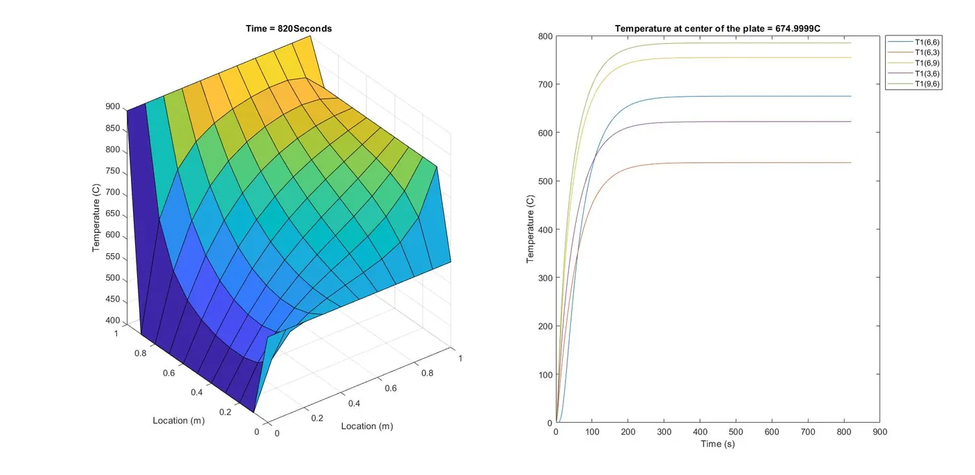
Jacobi method converged after 264 iterations and gauss seidel method took 140 iterations. The successive overrelaxation runs faster and only took 35 iterations to get the convergence. The optimum value of relaxation constant in this case is 1.5 which gives quick convergence. The contour plot of the graph shows the isothermal lines. The upper half the isotherms are more close and more heat is transferred because the isotherms are close. The bottom half of the plate involves less heat transfer. Isotherms are more close at plate corners. Explicit transient heat conduction results show the plate becomes the steady state in 810 seconds. After 810 seconds there is no change in temperature at any node is noticed. It is also found that the temperature profile at each node is different with respect to time. The magnitude of temperature at nodes increases and become steady in 810 seconds. The variation in temperature with time at five different locations is shown below. The steady state is achieved at all nodes at same time.

Program no : 01

%% PROGRAAM 01 
%% Title : Steady state heat conduction analysis using Jacobi, Guass-Seidel and Successive over relaxation iteration method

clear all
close all
clc
%% Steady State Heat Condition 
n = 11;
T = zeros(n,n); % Initiail temperature conditions
T(:,1) = 400;   % Bondary condition left
T(:,n) = 800;   % Bondary condition right
T(1,:) = 600;   % Bondary condition top
T(n,:) = 900;   % Bondary condition botom

T_old1 = T;T_old2 = T;T_old3 = T;
T1 = T;T2 = T;T3 = T;
XX = linspace(0,1,n);
YY = XX;
[x,y] = meshgrid(XX,YY);

%% Iteration Input Jacobi = 1, Gauss =2, Successive = 3

for method = 1:3
%% Jacobi Iteration
if method ==1
error1 = 9e9;
jcobi_iter = 0;
while error1 > 1e-4
    jcobi_iter =jcobi_iter + 1;
for       j = 2:(n-1)   
for       i = 2:(n-1)
    T1(i,j) = (T_old1(i-1,j)+T_old1(i+1,j)+T_old1(i,j-1)+T_old1(i,j+1))/4;
end
end
error1 = max(max(abs(T1-T_old1)));
T_old1 = T1;
subplot(3,3,1)
surf(x,y,T_old1)
title(['Jacobi : Iteration no. = ' num2str(jcobi_iter)])
xlabel('Location (m)')
ylabel('Location (m)')
zlabel('Temperature (C)')
colorbar
subplot(3,3,2)
pcolor(x,y,T_old1)
xlabel('Location (m)')
ylabel('Location (m)')
zlabel('Temperature (C)') 
subplot(3,3,3)
contour(x,y,T_old1)
xlabel('Location (m)')
ylabel('Location (m)')
zlabel('Temperature (C)') 
pause(0.01)
end
%% Gauss Iteration
elseif method ==2
       error2 = 9e9;
   gauss_iter = 0;
while error2 > 1e-4
   gauss_iter = gauss_iter + 1;
for j = 2:(n-1)  
for i = 2:(n-1)
    T2(i,j) = (T2(i-1,j)+T_old2(i+1,j)+T2(i,j-1)+T_old2(i,j+1))/4;
end
end
error2 = max(max(abs(T2-T_old2)));
T_old2 = T2;
subplot(3,3,4)
surf(x,y,T_old2)
title(['Gauss-Seidel : Iteration no = ' num2str(gauss_iter)])
xlabel('Location (m)')
ylabel('Location (m)')
zlabel('Temperature (C)')
colorbar
subplot(3,3,5)
pcolor(x,y,T_old2)
xlabel('Location (m)')
ylabel('Location (m)')
zlabel('Temperature (C)')
subplot(3,3,6)
contour(x,y,T_old2)
xlabel('Location (m)')
ylabel('Location (m)')
zlabel('Temperature (C)')
pause(0.01)
end
%% Succesive Over Relaxation
else
c = 2*cos(pi/n);    
w = 4/(2+sqrt(4-c^2));    % relaxation parameter
succover_iter = 0;
error3 = 9e9;
while error3 > 1e-4
    succover_iter =succover_iter + 1;
for       j = 2:(n-1)  
for       i = 2:(n-1)
    T3(i,j) =(1-w)*T3(i,j)+w*(T3(i-1,j)+T_old3(i+1,j)+T3(i,j-1)+T_old3(i,j+1))/4;
end
end
error3 = max(max(abs(T3-T_old3)));
T_old3 = T3;
subplot(3,3,7)
surf(x,y,T_old3)
title(['SORM : Iteration no. = ' num2str(succover_iter)])
xlabel('Location (m)')
ylabel('Location (m)')
zlabel('Temperature (C)')
colorbar
subplot(3,3,8)
pcolor(x,y,T_old3)
xlabel('Location (m)')
ylabel('Location (m)')
zlabel('Temperature (C)')
subplot(3,3,9)
contour(x,y,T_old3)
xlabel('Location (m)')
ylabel('Location (m)')
zlabel('Temperature (C)')
pause (0.01)
end
end
end

Program no. 02

Steady state heat conduction by Transient explicit

%% Program no 02
%% Title : Steady state heat conduction by Transient explicit
clear all
close all
clc

%% Transient Explicit
% Steady State Heat Condition 
n        = 11;
T        = zeros(n,n); % Initiai temperature conditions
T(:,1)   = 400;        % Bondary condition left
T(:,n)   = 800;        % Bondary condition right
T(1,:)   = 600;        % Bondary condition top
T(n,:)   = 900;        % Bondary condition botom
T_old1   = T;
T1 = T;
T_left   = [];
T_right  = [];
T_top    = [];
T_bottom = [];
XX       = linspace(0,1,n);
YY       = XX;
[x,y]    = meshgrid(XX,YY);
dt       = 1;          % Time step size 
alpha    = 0.001;      % Thermal diffusivity
dx       = XX(2)-XX(1);
T_centre = [];
index    = 0;
duration = [];
time     = 820;        % Analysis time
for t    = 1:time/dt
   index = index + 1;
duration = [duration index];
for j    = 2:(n-1)   
for i    = 2:(n-1)
T1(i,j)  = T_old1(i,j)+(alpha*dt/(dx^2))*(T_old1(i,j-1)+T_old1(i,j+1)+T_old1(i-1,j)+T_old1(i+1,j)-4*T_old1(i,j));
end
end 
T_old1 = T1;
subplot(1,2,1)
surf(x,y,T_old1)
title(['Time = ' num2str(index) 'Seconds'])
xlabel('Location (m)')
ylabel('Location (m)')
zlabel('Temperature (C)')
pause(0.001)
T_centre = [T_centre T1(6,6)];
T_left   = [T_left T1(6,3)];
T_right  = [T_right T1(6,9)];
T_top    = [T_top T1(3,6)];
T_bottom = [T_bottom T1(9,6)];
subplot(1,2,2)
plot(duration,T_centre,duration,T_left,duration,T_right,duration,T_top,duration,T_bottom)
xlabel('Time (s)')
ylabel('Temperature (C)')
title(['Temperature at center of the plate = ' num2str(T1(6,6)) 'C'])
legend('T1(6,6)','T1(6,3)','T1(6,9)','T1(3,6)','T1(9,6)')
pause(0.001)
end

Program no. 03

Steady state heat conduction by transient implicit

%% Program no. 03
%% Title : Steady state heat conduction by transient implicit
clear all
close all
clc
%% Steady State heat condition 
n      = 11;
T      = zeros(n,n); % Initiail temperature conditions
T(:,1) = 400;        % Bondary condition left
T(:,n) = 800;        % Bondary condition right
T(1,:) = 600;        % Bondary condition top
T(n,:) = 900;        % Bondary condition botom
T_old1 = T;   T_old2 = T;  T_old3 = T;
T1     = T;       T2 = T;      T3 = T;
T_1    = T;       T_2= T;      T_3= T;
XX     = linspace(0,1,n);
YY     = XX;
[x,y]  = meshgrid(XX,YY);
dt     = 10;         % Time step size 
alpha  = 0.001;      % Thermal diffusivity
dx     = XX(2)-XX(1);
time   = 200;        % Total time for which the analysis is performed
k      = alpha*dt/(dx^2);
% Iteration Input Jacobi = 1, Gauss = 2, Successive = 3
for method = 1:3
if method  == 1
%% Jacobi Iteration Method
jacobi_iter = 0;
for t       = 1:time/dt
    error_1  = 9e9;
while error_1 > 1e-4
jacobi_iter = jacobi_iter +1; 
for j       = 2:(n-1)   
for i       = 2:(n-1)
    T1(i,j) = T_1(i,j)/(1+4*k)+(k/(1+4*k))*(T_old1(i,j-1)+T_old1(i,j+1)+T_old1(i-1,j)+T_old1(i+1,j));
end
end
error_1 = max(max(abs(T1-T_old1))); 
T_old1 = T1;
subplot(3,1,1)
surf(x,y,T_1)
title(['Jacobi : Iteration no. = ' num2str(jacobi_iter) ' & Time = ' num2str(time) 'Seconds'])
xlabel('Location (m)')
ylabel('Location (m)')
zlabel('Temperature (C)')
pause(0.03)
end
T_1 = T1;
end
elseif method == 2
%% Gauss-Seidel iteration method
Gauss_iter  = 0;
for t       = 1:time/dt
    error_2  = 9e9;
while error_2 > 1e-4
    Gauss_iter = Gauss_iter +1;
for j       = 2:(n-1)   
for i       = 2:(n-1)
    T2(i,j) = T_2(i,j)/(1+4*k)+(k/(1+4*k))*(T2(i,j-1)+T_old2(i,j+1)+T2(i-1,j)+T_old2(i+1,j));
end
end
error_2 = max(max(abs(T2-T_old2))); 
T_old2 = T2;
subplot(3,1,2)
surf(x,y,T_2)
title(['Gauss-Seidel : Iteration no. = ' num2str(Gauss_iter) ' & Time = ' num2str(time) 'Seconds'])
xlabel('Location (m)')
ylabel('Location (m)')
zlabel('Temperature (C)')
pause(0.03)
end
T_2 = T2;
end
else
%% Succesive Over Relaxation Method (SORM)
         w = 1.5;  % relaxation parameter
Succ_iter  = 0;
for      t = 1:time/dt
   error_3 = 9e9;
while error_3 > 1e-4
    Succ_iter = Succ_iter +1;
for j       = 2:(n-1)   
for i       = 2:(n-1)
    T3(i,j) =(1-w)*T3(i,j)+w*(T_3(i,j)/(1+4*k)+(k/(1+4*k))*(T3(i,j-1)+T_old3(i,j+1)+T3(i-1,j)+T_old3(i+1,j)));
end
end
error_3 = max(max(abs(T3-T_old3))); 
T_old3 = T3;
subplot(3,1,3)
surf(x,y,T_3)
title(['SORM : Iteration no. = ' num2str(Succ_iter) ' Time = ' num2str(time) 'Seconds'])
xlabel('Location (m)')
ylabel('Location (m)')
zlabel('Temperature (C)')
pause(0.03)
end
T_3 = T3;
end    
end
end