Week 5 - Rayleigh Taylor Instability

Rayleigh Taylor instability:

It is the instability caused at the interface of the two fluids of different densities when the lighter fluid pushes the heavier fluid. Some examples of Rayleigh taylor instability are water suspended on top of oil, mushroom clouds formation from nuclear explosion and volcanic eruptions, etc.

CFD models based on mathematical analysis of Rayleigh Taylor waves:

1. Richtmyer-Meshkov Instability(RMI): The Richtmyer–Meshkov instability (RMI) occurs when two fluids of different density are impulsively accelerated. Normally this is by the passage of a shock wave. The development of the instability begins with small amplitude perturbations which initially grow linearly with time. This is followed by a nonlinear regime with bubbles appearing in the case of a light fluid penetrating a heavy fluid, and with spikes appearing in the case of a heavy fluid penetrating a light fluid. A chaotic regime eventually is reached and the two fluids mix. This instability can be considered the impulsive-acceleration limit of the Rayleigh–Taylor instability.

2. Kelvin-helmholtz instability: The Kelvin–Helmholtz instability (after Lord Kelvin and Hermann von Helmholtz) typically occurs when there is velocity shear in a single continuous fluid, or additionally where there is a velocity difference across the interface between two fluids. A common example is seen when wind blows across a water surface; the instability constant manifests as waves. Kelvin-Helmholtz instabilities are also visible in the atmospheres of planets and moons, such as in cloud formations on Earth or the Red Spot on Jupiter, and the atmospheres (coronas) of stars, including the sun's.

3. Plateau-Rayleigh Instability: The Plateau–Rayleigh instability, often just called the Rayleigh instability, explains why and how a falling stream of fluid breaks up into smaller packets with the same volume but less surface area. It is related to the Rayleigh–Taylor instability and is part of a greater branch of fluid dynamics concerned with fluid thread breakup. This fluid instability is exploited in the design of a particular type of ink jet technology whereby a jet of liquid is perturbed into a steady stream of droplets.

The driving force of the Plateau–Rayleigh instability is that liquids, by virtue of their surface tensions, tend to minimize their surface area. A considerable amount of work has been done recently on the final pinching profile by attacking it with self-similar solutions.

Geometry:

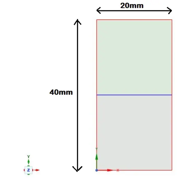
The following 2D geometry is made using space claim with the given dimensions.

Meshing

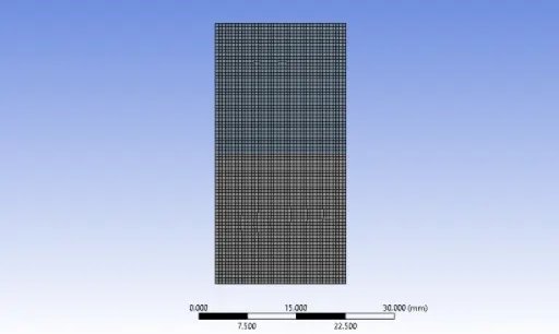
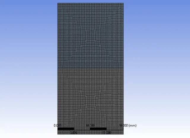
1.Coarse Mesh (Element size = 0.5mm)

Fluent settings:

Pressure based solver

Transient simulation

Gravity= 9.81 m/s in -y direction

VOF model

Implicit formulation method

Water on upper half, air on lower half

Patching should be done.

Time step size= 0.005

2.Fine Mesh (Element size = 0.25mm)

3. User defined material, element size = 0.25mm

Results:

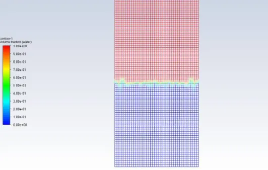
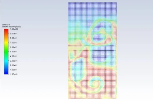
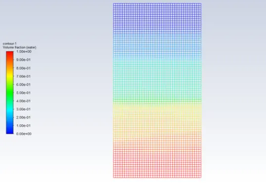
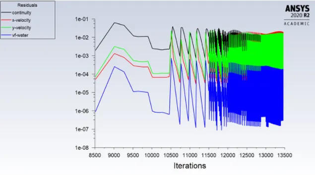
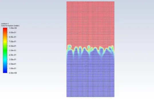
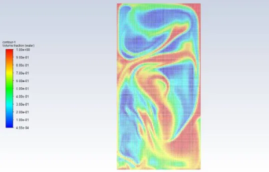
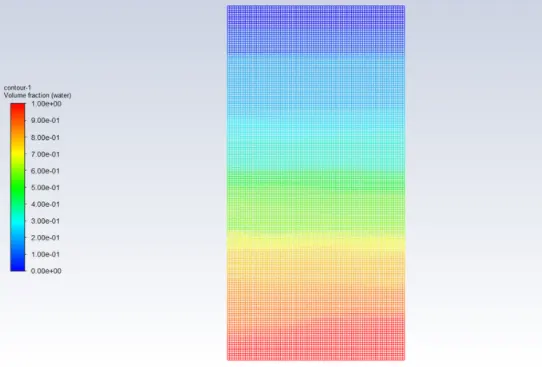
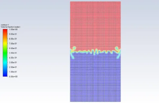
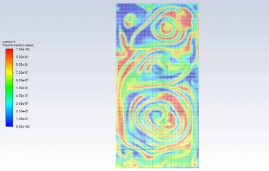
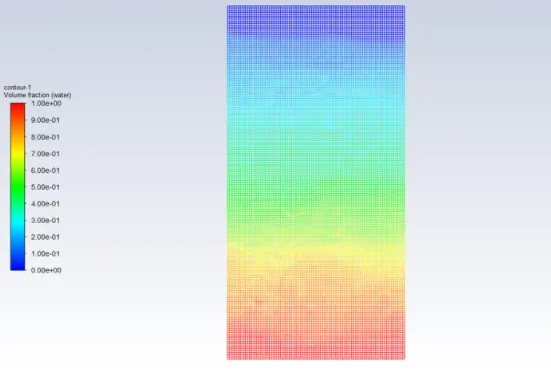
1. For the coarse mesh size the instability is not properly visible but for fine mesh it is clear.
2. Coarse mesh size have less nodes so the solution takes less time.
3. Fine mesh size have more nodes resulting in more time.
4. When the atwood number is around 0 the stability takes the form of symmetric fingers of fluid whereas when atwood number is around 1 the heavier fluid takes the form of large bubble like plumes.
5. At the end of the simulation, the air and water are not fully separated and diffusion can be seen around the interface.

Atwood Number:

The Atwood number ( A) is a dimensionless number in fluid dynamics used in the study of hydrodynamic instabilities in density stratified flows. It is a dimensionless density ratio defined as Atwood number is an important parameter in the study of Rayleigh–Taylor instability and Richtmyer–Meshkov instability.

The Atwood number (A) is a dimensionless number in fluid dynamics used in the study of hydrodynamic instabilities in density stratified flows. It is a dimensionless density ratio defined as

where

= density of heavier fluid

= density of lighter fluid

Atwood number for water-air simulation:

Water density = 998.2 kg/m3

Air density = 1.225 kg/m3

A= 0.997

Atwood number for water-air simulation:

Water density = 998.2 kg/m3

Air density = 1.225 kg/m3

A= 0.428

When the atwood number is less, the stability takes the form of symmetric fingers of fluid and fluid is found to be more stable whereas when atwood number is more the heavier fluid takes the form of large bubble like plumes and more instablity takes palce in fluid.