Week 5 - Rayleigh Taylor Instability
Aim: To simulate Rayleigh-Taylor Instability, and track the development of interface as fluids move to stable configration. Perform the simulation for varying mesh sizes to spot the variation in disturbances.
Introduction
When two fluids of different densities are superimposed on one another or accelerated towards each other, the instability of the plane interface as it occurs is called Rayleigh-Taylor Instability.
Even in stable configration, a slight displacement of surface results in waves travelling horizantally on the surface or interface. These waves let the lighter fluid to rise and heavier fluid to fall such as the potential energy of the system will decrease to its minumum. This essentially, defines the behaviour of the interface.
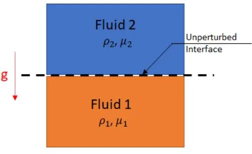
Fig 1: Rayleigh-Taylor Instability
ρ2 > ρ1 => Unstable Configration
ρ2 < ρ1 => Stable Configration
Atwood Number: It is a dimensionless number which describes the nature of interface. It is denoted by A and can be defined as:
A = (ρ2 - ρ1)/ (ρ2 + ρ1)
A>0 => Unstable Configration
A<0 => Stable Configration
Practical Significance of Rayleigh-Taylor Instability
Such dymanic phenomena occurs in diverese processes and thus it is important to understand such an unstable process. Some of the areas where it is important are as follows:
Astrophysics:
RT instability plays a vital role in astrophysical phenomena, particularly in the dynamics of supernovae explosions, where the mixing of materials with different densities influences the evolution of the explosion.
It also contributes to the mixing of elements in stars and can impact the formation and evolution of galaxies.
Inertial Fusion Energy (IFE):
Similar to ICF, RT instability is a concern in inertial fusion energy research. It can affect the efficiency and stability of the fusion reaction in potential future energy production systems.
Plasma Physics:
RT instability is observed in plasma systems, such as magnetic confinement devices like tokamaks. It can influence the performance and stability of these devices by affecting plasma confinement and transport.
Material Mixing in Engineering Applications:
In engineering contexts, Rayleigh-Taylor instability can impact the mixing of materials in various processes, such as the injection of one fluid into another, as seen in fuel injection systems or certain manufacturing processes.
Understanding and controlling RT instability is crucial for optimizing these processes and ensuring uniform material distribution.
Environmental Flows:
In environmental sciences, RT instability can affect the mixing of fluids in natural systems, such as the interface between freshwater and saltwater in estuaries or the dispersion of pollutants in water bodies.
Aerospace and Defense:
RT instability can influence the behavior of shock waves in supersonic and hypersonic flows, impacting the aerodynamics of aerospace vehicles and the design of reentry vehicles.
CFD Models based on the Mathematical Aspects of Rayleigh Taylor Instability
The following are some CFD models that are used in Rayleigh-Taylor Instability:
Level Set Method:
The Level Set method is often employed to track the evolution of the interface between the two fluids.
A level set function is used to represent the interface, and its evolution is determined by solving a transport equation. This method allows for capturing the complex and dynamic behavior of the Rayleigh-Taylor interface.
Volume-of-Fluid (VOF) Method:
VOF is a popular technique for simulating free-surface flows, including Rayleigh-Taylor instability.
It tracks the volume fractions of different fluids within each computational cell, enabling the modeling of fluid interfaces and their interactions.
Smoothed Particle Hydrodynamics (SPH):
SPH is a mesh-free Lagrangian method that has been adapted for Rayleigh-Taylor simulations.
It represents the fluid as a collection of particles, and the inter-particle interactions are calculated to simulate the fluid flow and mixing.
Implicit Large Eddy Simulation (ILES):
ILES is a turbulence modeling approach that resolves large-scale turbulent structures implicitly.
It is often combined with other methods to simulate the turbulent nature of Rayleigh-Taylor instability.
Solving and Modelling Approach
We will approach it as a Multi-phase problem which is subjected to the gravitational field. We will place water as heavier fluid on top of the lighter fluid air. We will setup the transient solver and run the simulation for a a fixed time step. We will also setup contours of volume fraction to investigate the variation of the interface and as the interface gets stable we will consider that as out final result. The aim is not to get to a result in here but it is about to investigate a dynamic process as it unfolds. We will use the following steps in our solving and modelling approach:
1. Geometry Creation: We will create a simple geometry in Ansys Space Claim
2. Structured Mesh Generation: Due to the simplicity of the geometry, a hexa mesh is most suited as it makes solver easier to converge.
3. Solver Setup in Ansys-Fluent: Here we will set up the solver that will run the simulation. We will use Parallel Processing with Double Precision, this runs the simulation faster.
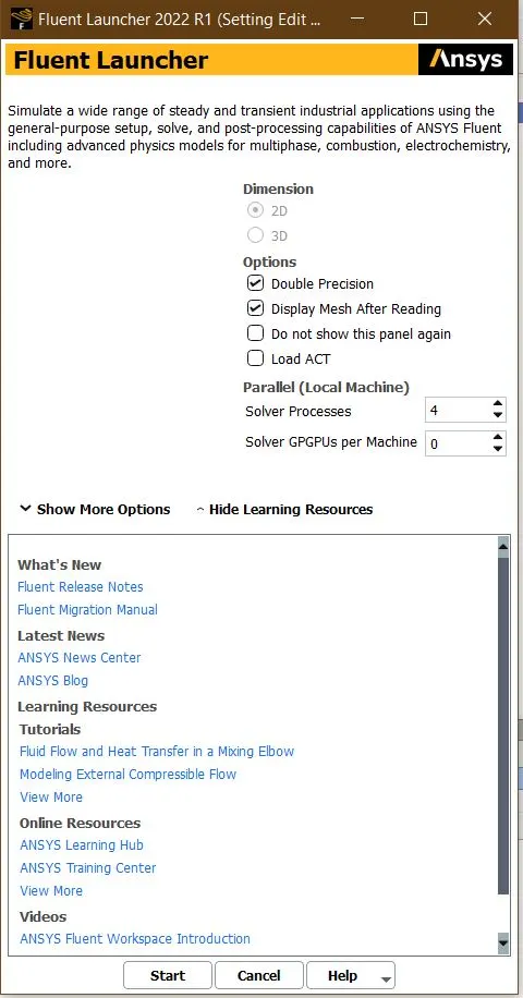
Fig 2: Fluent Setup
Pre-Processing
Step 1: We will create a simple geometry two 20x20 mm2 squares on top of one another, we will join the intersection of the two squares with share command from workbench in Space claim. This will lead to the creation of conformal mesh in meshing.
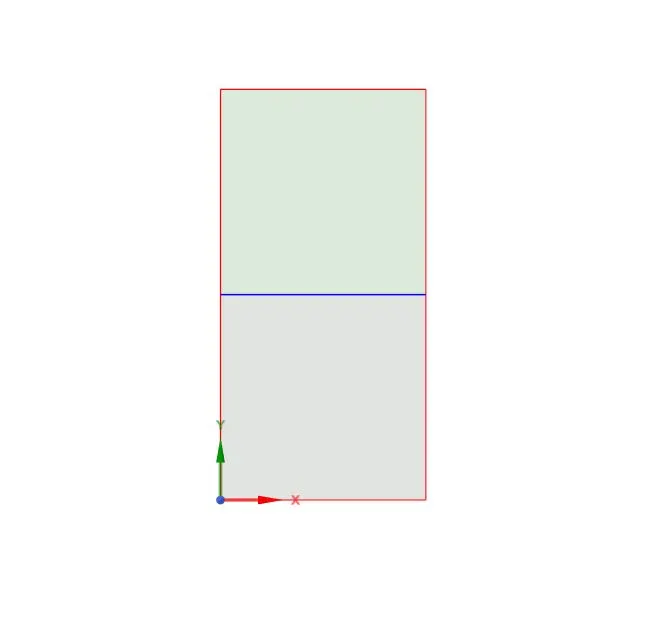
Fig 3: Setting up the Physical Domain
Step 2: We will perform structured meshing over this physical domain to get our computational domain.
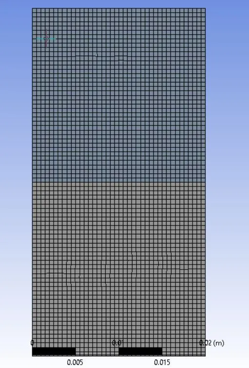
Fig 4: Setting up the Computational Domain
Step 3: We will now move to Fluent to set up the solver.
First of all we set up the General Settings. We are going to use a Pressure-based Transient solver with Gravitational effects. The value of g is taken negative since it is acting opposite to the y-coordinate in our setup.
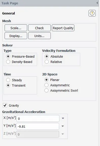
Fig 5: General Settings
Secondly, we will setup up the turbulence model. Since, the flow is going to be Laminar we will use the default Kω-SST model.
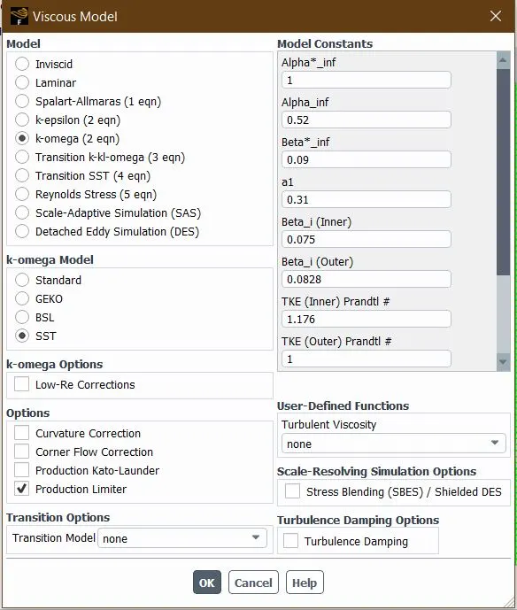
Fig 6: Selection of Viscous Model
Thirdly, we will setup the multi-phase model. We will use Volume-Of-Fluid approach which is suited for multiphase flows and we will use implicit scheme.
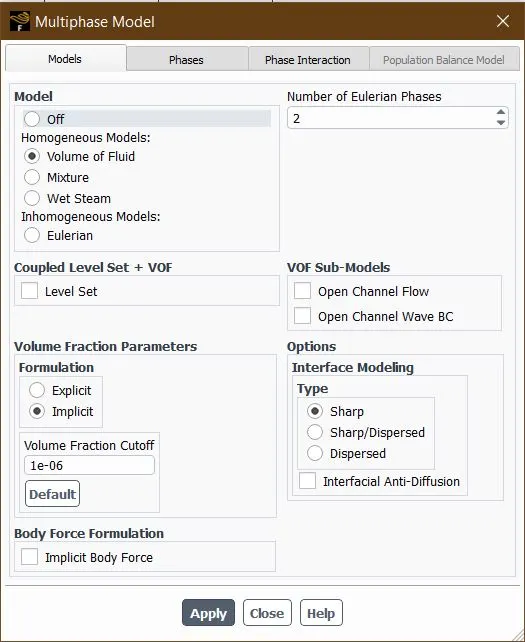
Fig 7: Selection of Multi-Phase Model
Fourthly, we will set up the fluid. the heavier fluid as water and lighter fluid as air.
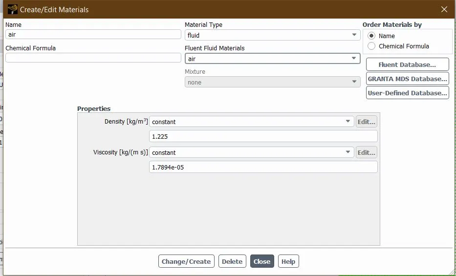
Fig 8: Material Selection
Now we will initialize the solution using Standard approach. and we will patch the surfaces under volume fraction. We will take water and associate volume-fraction as 1 and under water we will put volume fraction of air as 0.
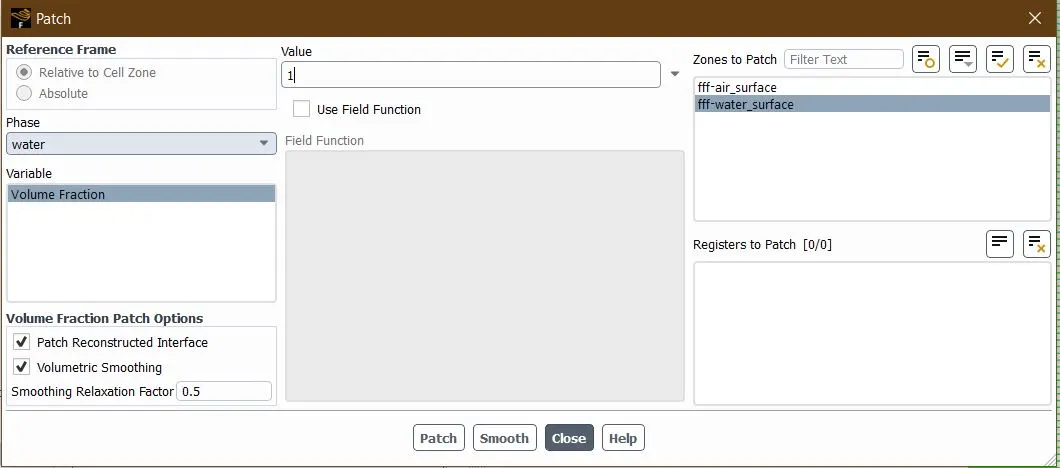
Fig 9: Patching volume fraction of water in water surface
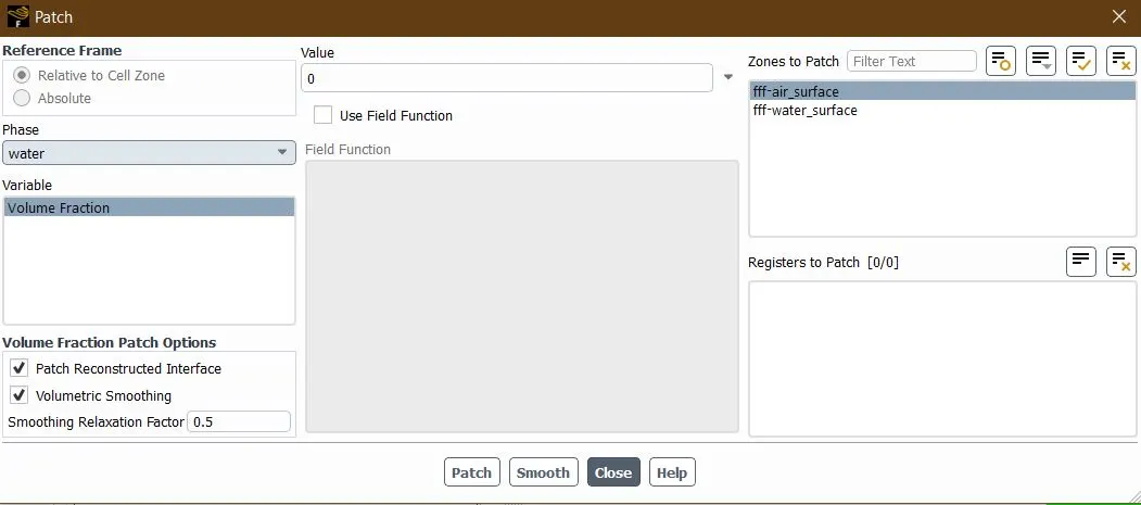
Fig 10: Patching volume fraction of air in water surface
Finally we will run the solver with following parameters:
Time Step Size = 0.005 seconds
Number of Time Steps = 1500
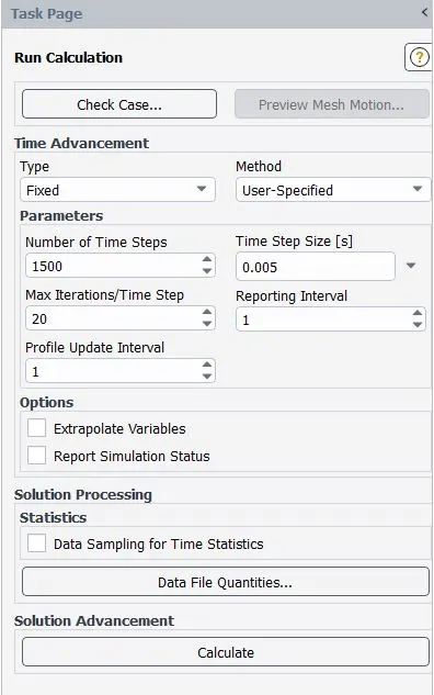
Fig 11: Calculation setup
Each Mesh Case and Post Processing of Results
1. Baseline Mesh
Element size = 0.5 mm
Number of Elements = 3200
Mesh
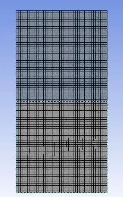
Fig 12: Baseline Mesh
Residuals
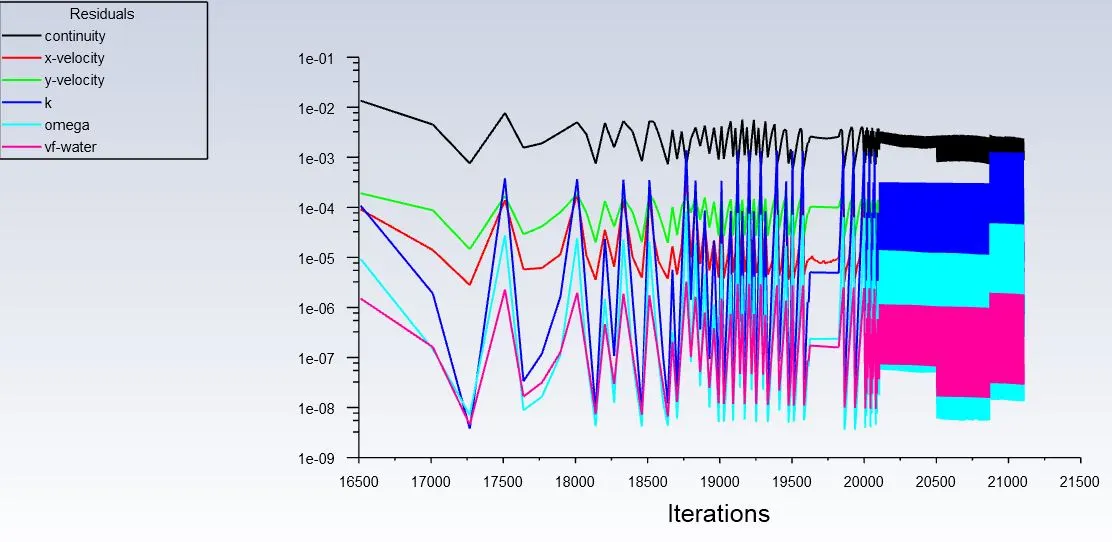
Fig 13: Baseline Mesh Residuals
Simulation Video Link
https://drive.google.com/file/d/1aIW-7U-v7tchkDJM4yEfosBy0Y9ZqeKg/view?usp=sharing
2. Refined Mesh
Element size = 0.15 mm
Number of Elements = 35380
Mesh
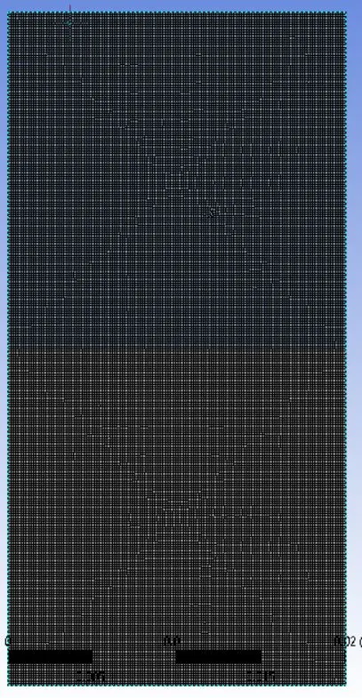
Fig 14: Refined Mesh
Residuals
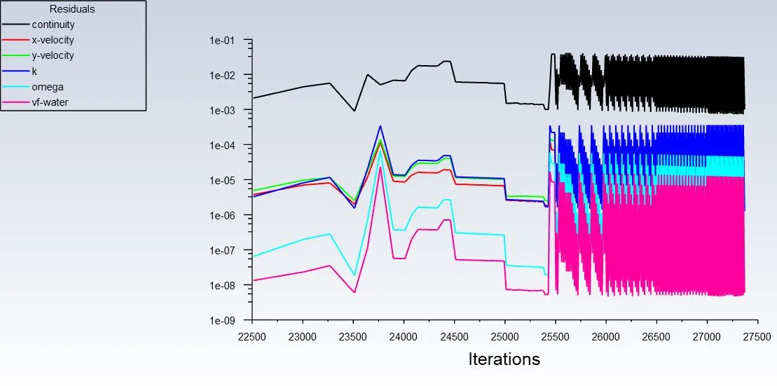
Fig 15: Refined Mesh Residuals
Simulation Video Link
https://drive.google.com/file/d/1cpPf5CUG9z-ht_i5EIyktmeWCNgeSrks/view?usp=sharing
3. Mesh with User-defined fluid
Element size = 0.15 mm
Number of Elements = 35380
MESH
Fig 16: User Defined Fluid Mesh
Residuals
Fig 17: User Defined Fluid Residulas
Simulation Video Link
https://drive.google.com/file/d/1q12R1PmPJc3KfmWkoz5ZCT3DFBUGKn_7/view?usp=sharing
Atwood Number Clculation
[ρ1-ρ2ρ1+ρ2]">A = (ρ2 - ρ1)/ (ρ2 + ρ1)
For CASE 1 and 2:
ρ1">ρ1�1 = 998.2kgm3">kgm3���3
ρ2">ρ2�2 = 1.225kgm3">kgm3���3
A = [998.2-1.225998.2+1.225]">[
1.225 - 998.21.225 + 998.2][998.2-1.225998.2+1.225]
A = -0.9975
For CASE 3:
ρ1">ρ1�1 = 998.2kgm3">kgm3���3
ρ2">ρ2�2 = 400kgm3">kgm3���3
A = [998.2-400998.2+400]">[
400 - 998.2
400 + 998.2][998.2-400998.2+400]
A = - 0.4278
Observations
The growth of instability can be classified in three stages:
1. Linear Stablity
The interface keeps falling down due the higher weight of water and air keeps getting pumped up from the sides of the wall. Due to surface tension, air can not rupture the water surface as a reaction to getting compressed by water, instead it peeps out from the outer sides.
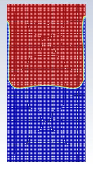
Then, the air streams moving up merges together at the top which leads to formation of water inside air like a bubble.
2. Mushroom Head Falling
We call this stage mushroom head because at the lower portion of water there is a formation of a symmetrical mushroom head.
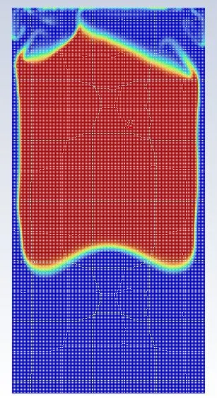
Now as this mushroom head reaches at the lower portion of the geometry, it entraps an air-bubble.
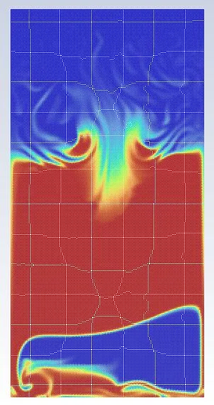
This entraping causes increases in energy of the bubble as it keeps getting compressed by the falling water. As this bubble escapes, it stirrs up the whole section into an unprecidented wave motion.
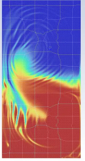
3. Long Term Evolution due to bubble merging and mixing
Now as water and air are at their places, the whole system is trying to relax and the interface can be seen as interchanging bubbles of both liquids which finally leads to stability
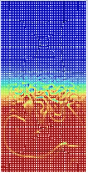
Rayleigh-Taylor Instability comparision with a User Defined Fluid with decreased density.
1. Linear Stability
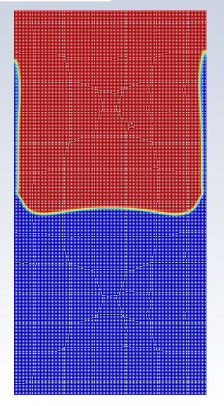
Case 2 Case 3
No significant difference at this stage
2. Mushroom Head Falling
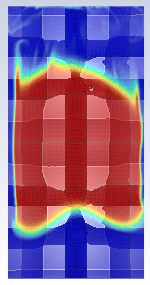
Case 2 Case 3
The mushroom head for case 2 is largely a symmetrical.
3. Long term evolution due to bubble merging and mixing
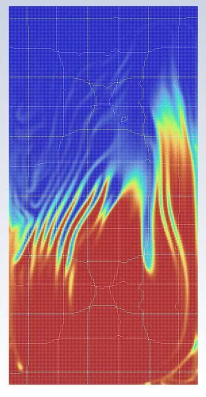
Case 2 Case 3
The turbulent wave motion is more precedented for case 2 due to the lower value of Atwood Number.
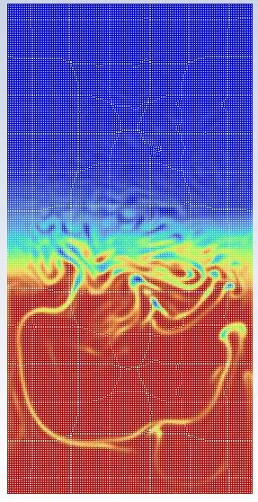
Case 2 Case 3
The interface is taking longer to stabalize for case 2 as larger number of air bubbles are trapped under water surface, this is also due to the lower value of Atwood Number.
Due to this unprecedented wave motion that is observed in Rayleigh Taylor instability, a steady state solver will not yield correct results as the flow parameters are continously changing with respect to time.
References
Rayleigh-Taylor Instability Notes J. Oakley