Week 5 - Rayleigh Taylor Instability

RAYLEIGH TAYLOR INSTABILITY

AIM:

To conduct the Rayleigh Taylor Simulation

Answer for Ques No:1

LEARNINGS:

Rayleigh-Taylor instability is a disturbance caused by the denser fluid forcefully occupying the lighter fluid. It is seen in natural and engineered systems like inertial confinement fusion, specific mixing of fluids and even supernova explosions. The dynamics of Rayleigh instability are made more accessible by Numerical simulation.

Growth of Simulation:

Simulations reveal the growth of initial minor disturbances at the interface between the two fluids. These agitations grow exponentially over time, leading to the development of intricate structures like spikes and bubbles. The evolving interface between the two fluids results in bubbles of the lighter fluid and spikes of the heavier fluid. The interplay between buoyancy and surface tension determines the structures and characteristic shapes and sizes.

Mixing and Turbulence: Rayleigh-Taylor instability is a source of mixing between the two fluids. Simulations provide insights into the evolution of turbulence and the resulting mixing efficiency. Understanding mixing is crucial in applications like inertial confinement fusion, where achieving a uniform fuel mix is essential.

Shock Wave Formation:

In specific scenarios, the growth of Rayleigh-Taylor instability can lead to the development of shock waves. Simulations help study these shock waves' formation, propagation, and interaction, which is essential in various astrophysical and engineering contexts.

Influence of Viscosity and Diffusivity:

Simulations allow researchers to explore the effects of viscosity and diffusivity on the evolution of Rayleigh-Taylor instability. These properties can significantly alter the growth rates and morphology of the instability.

Parametric Studies:

Simulations enable researchers to conduct parametric studies by varying initial conditions, material properties, and other parameters. This helps identify the key factors influencing instability and its evolution.

Interfacial Mixing Models:

Simulations contribute to the development of improved models for interfacial mixing, which are essential for accurate predictions of the evolution of the instability and its impact on the overall system.

Navier-Stokes Equations:

The foundation of CFD simulations lies in the Navier-Stokes equations, which describe the conservation of mass, momentum, and energy in fluid flow. These equations form the basis for modelling fluid motion and are central to understanding Rayleigh-Taylor instability.

Interface Tracking/Representation:

In the context of Rayleigh-Taylor simulations, the interface between the two fluids needs to be tracked accurately. Various numerical methods, such as volume-of-fluid (VOF) or level-set methods, represent and follow the evolving interface over time.

Density and Pressure Formulations:

The density and pressure formulations in the CFD model are adapted to account for the stratification of the two fluids. The density contrast between the lighter and heavier fluids and their dynamic interaction is crucial for capturing the essence of Rayleigh-Taylor instability.

Buoyancy and Acceleration Terms:

Rayleigh-Taylor instability is driven by buoyancy forces resulting from the acceleration of one fluid into another. The mathematical models include terms that represent the buoyancy and acceleration effects, allowing the CFD solver to simulate the growth and evolution of the instability.

Turbulence Models:

Turbulence is inherent in Rayleigh-Taylor flows, especially as the instability evolves and leads to the formation of complex structures. CFD models incorporate turbulence models, such as Reynolds-averaged Navier-Stokes (RANS) or large-eddy simulation (LES), to account for turbulent mixing and enhance the accuracy of predictions.

Energy and Heat Transfer:

Energy and heat transfer between the fluids may be critical depending on the application. CFD models include heat conduction and convection to capture temperature variations associated with the Rayleigh-Taylor instability, especially in scenarios like inertial confinement fusion.

Validation and Calibration:

Mathematical models are validated and calibrated against experimental data to ensure that the CFD simulations accurately represent the physical phenomena. This process involves adjusting model parameters and numerical settings to match observed behaviours.

High-Performance Computing (HPC):

Rayleigh-Taylor simulations can be computationally demanding, especially when dealing with complex, three-dimensional flows and satisfactory spatial resolutions. High-performance computing techniques are often employed to handle the computational load and achieve accurate results within a reasonable timeframe.

Parametric Studies:

CFD models allow researchers to conduct parametric studies by varying initial conditions, fluid properties, and other parameters. This flexibility is essential for exploring the sensitivity of the Rayleigh-Taylor instability to different factors.

Overall, CFD models for Rayleigh-Taylor instability involve adapting the fundamental fluid dynamics equations to capture this phenomenon's specific characteristics. This includes accurately representing fluid interfaces, considering buoyancy and acceleration effects, including turbulence models, and validation against experimental data. The goal is to provide a computational framework that replicates the real-world behaviour of Rayleigh-Taylor waves and aids in understanding, predicting, and optimizing systems affected by this fluid instability. Simulations of Rayleigh-Taylor instability provide valuable insights into the complex fluid dynamics associated with the phenomenon. These learnings contribute to understanding fundamental physical processes and have practical implications for various scientific and engineering applications.

Answer for Question 2

Rayleigh Taylor instability simulation:

I made the assumptions according to the question. The base mesh is 0.5mm, and it should be further refined. The refined mesh values are 0.35 mm and 0.25 mm, respectively. Apart from the mesh sizes, the procedure followed the same for the entire procedure.

A) GEOMETRY:

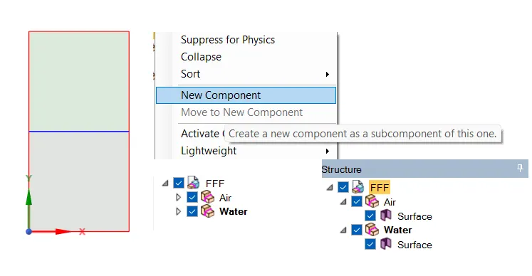
• Squares are drawn individually and pulled to the new component.
• The procedure is followed twice for different component
• Topology is shared, which is indicated in the figure.
• Selecting a plane is most important for further geometry continuation.

Figure A (1):

B) MESH PART:

• Basic mesh from the workbench.
• For different cases, particularly 0.5mm, 0.35 mm and 0.25 mm.
• Element sizes are varied, and results are observed.

Figure B (1):

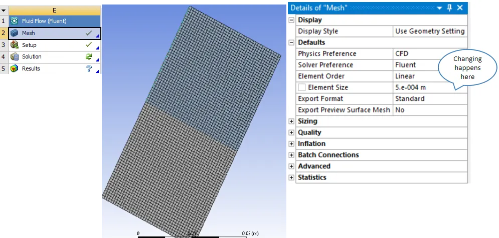
For 2 different mesh sizes, with the base mesh being 0.5 mm.

C)FLUENT PART:

• General functions like Pressure, Transient condition, and Gravity are enabled.
• Gravity is about 9.81 ms^-2 and is acting downwards, so the values are taken as negative.
• Viscous flow is Laminar.
• Multiphase model for volume of fluid with two Eulerian phases.
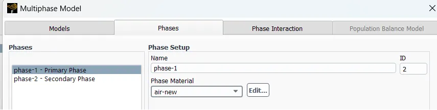
• Phases are assigned accordingly.
• The value of water is taken from the fluent database of materials and copied and assigned to phase 2.
• The user-defined values are changed by copying the value of air, and the density and viscosity values are changed according to the given conditions.
• Standard initialisation is done.
• Patch the values for water and air as 1 and 0 from the variable volume fraction considering the phase as water.
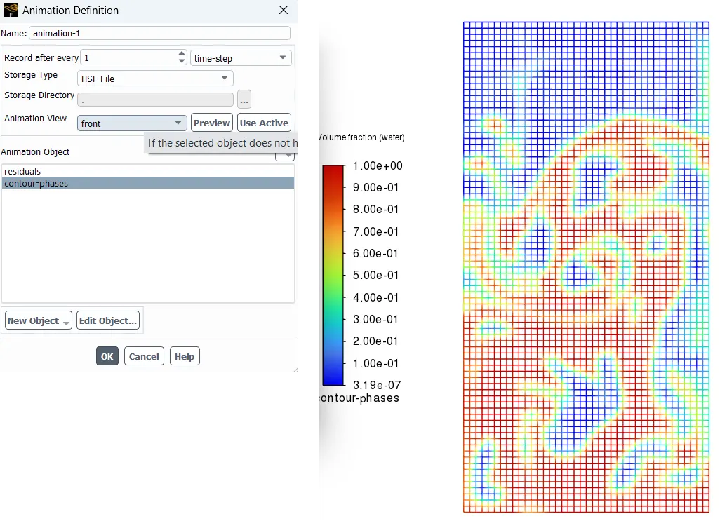
• Successful patches to respective zones create contours for phases (water) and their respective Animation.
• Run calculations.

REASON for Sub Questions:

Transient condition is preferred for calculating or capturing the instabilities which are not predictable. Most probably, the conditions that do not possess unique agitations and are continuously time-dependent are solved using transient conditions. The steady state is used only for the solutions that possess functions invariant with time.

Since the simulation involves capturing instabilities which are changing unpredictably as a function of time, the transient approach is preferred over the steady-state approach. 

Figure (c) 1:

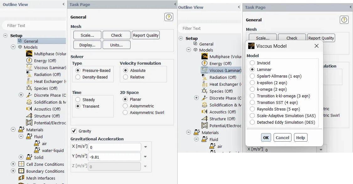
Figure (c) 2:

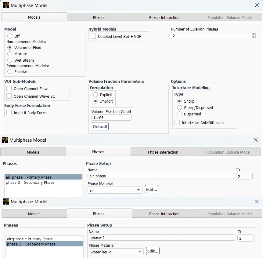
Figure (c) 3:

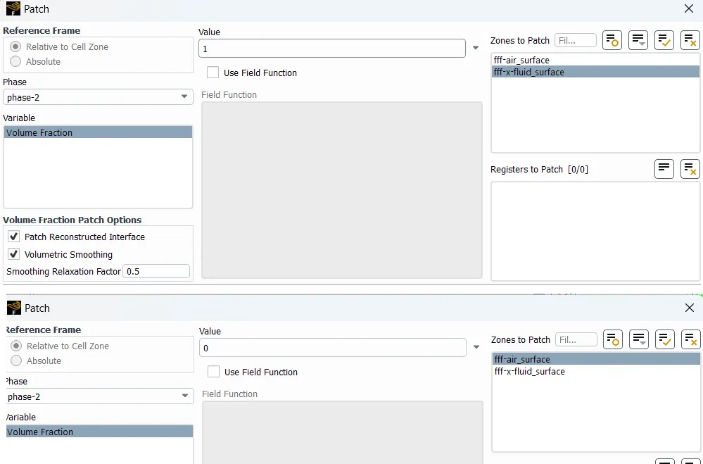
Figure (c) 4:

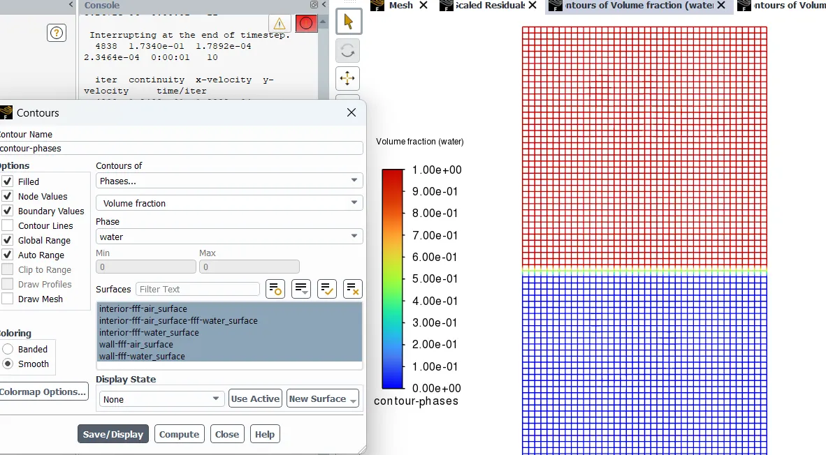
Figure (c) 5:

For User-defined fluid:

Comparing Results with Animation:

https://drive.google.com/drive/folders/1O1gRQMwRJXaBDRKVWwcwKH_mP5sKZRCI?usp=sharing

Animations for all cases are compiled in a folder and uploaded to Google Drive.

Results by Observation:

Finer mesh captures the instability better than the coarse mesh, but it takes more time for the heavier fluid to settle down. So, it is computationally expensive but produces results with better accuracy.

ATWOOD NUMBER:

The Atwood number (A) is a dimensionless parameter used in fluid dynamics to characterise the behaviour of fluids in a gravitational field when there is a density difference between two fluids. It is named after the British engineer George Atwood, who studied the motion of fluids in a gravitational field. The Atwood number quantifies the relative importance of buoyancy forces compared to inertial forces in the flow. It is often used in studying phenomena such as Rayleigh-Taylor instabilities, where the density difference between two fluids leads to complex flow patterns. The Atwood number helps predict the behaviour of these flows and is a crucial parameter in understanding the dynamics of multiphase fluid systems.

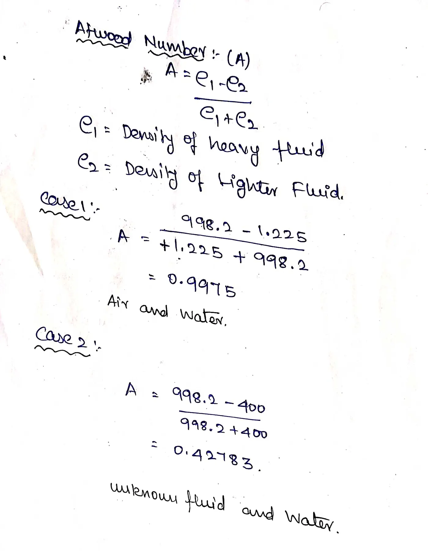
The Atwood number plays a significant role in the behaviour of instabilities, particularly in the context of fluid dynamics and the study of Rayleigh-Taylor instability. This instability occurs at an interface between two fluids of different densities when the heavier fluid is placed above the lighter one. The variation in the Atwood number (A) affects the behaviour of this instability in the following ways:

• Instability Growth Rate:

• A higher Atwood number implies a more significant density difference between the two fluids.

• This density difference directly influences the growth rate of the instability.

• More significant Atwood numbers often lead to faster growth of the Rayleigh-Taylor instability.

• Transition to Turbulence:

• The Atwood number influences the transition from a linear to a nonlinear stage and eventually to turbulent mixing.

• Higher Atwood numbers can result in an earlier transition to turbulence, leading to more complex and chaotic fluid motion.

• Amplitude of Perturbations:

• The amplitude of initial perturbations at the interface between the two fluids is affected by the Atwood number.

• Higher Atwood numbers typically lead to more significant initial perturbations.

• Flow Patterns:

• The Atwood number influences the specific flow patterns and structures that develop during the instability.

• The instability might manifest in more regular structures for lower Atwood numbers, while higher Atwood numbers can lead to more complex and irregular patterns.

• Mixing Efficiency:

• The Atwood number affects the efficiency of mixing between the two fluids.

• Higher Atwood numbers generally result in more efficient mixing due to the more vital buoyancy forces driving the fluid motion.

• Stability Threshold:

• The Atwood number is used to determine the stability of the system. A positive Atwood number A > 0 implies an unstable configuration, while a negative A < 0 indicates a stable configuration.

Unknown fluid is less in Atwood number when compared, so it possesses a very slow response in RT Stability. Understanding the behaviour of the Rayleigh-Taylor instability, as influenced by the Atwood number, is crucial in various scientific and engineering applications, including astrophysics, inertial confinement fusion, and the study of fluid dynamics in the presence of gravity. Researchers use experiments, numerical simulations, and theoretical analyses to investigate the effects of Atwood number variations on the instability and to gain insights into related phenomena.

��=�2−�1�avg⋅��,