Week 5 - Rayleigh Taylor Instability

Aim 

To verifying the Rayleigh Stablity in CFD simulations

Objective

• Explain different CFD models used for solving Rayleigh Taylor Instability problems
• Perform a Rayleigh Taylor instability analysis using the Volume of Fluid (VOF) multiphase model for air and water for two different mesh element sizes.
• Repeat the process for water and user-defined material with density = 400 kg/m3, viscosity = 0.001 kg/m-s, and compare the behaviour.
• Define the Atwood number and derive it for each case. Explain the effect of Atwood number on instability.

Introduction

•  In this project, we are going to perform the two dimensional simulation for two immiscible fluids that have different densities. Initially, the fluid with high density is placed at the top region while the fluid having lesser density at the bottom. Due to gravity, the heavy dense fluid flows downwards making the less dense fluid to go up. This causes the Rayleigh Taylor instability between the interface of those two fluids. This instability is captured from this simulation which set to run at transient state.

Theory

Rayleigh -Taylor instability

The Rayleigh–Taylor instability, or RT instability is an instability of an interface between two fluids of different densities which occurs when the lighter fluid is pushing the heavier fluid. Examples include the behaviour of water suspended above oil in the gravity of Earth, mushroom clouds like those from volcanic eruptions and atmospheric nuclear explosions, supernova explosions in which expanding core gas is accelerated into denser shell gas, instabilities in plasma fusion reactors and inertial confinement fusion.

  As the RT instability develops, the initial perturbations progress from a linear growth phase into a non-linear growth phase, eventually developing "plumes" flowing upwards (in the gravitational buoyancy sense) and "spikes" falling downwards. In the linear phase, the fluid movement can be closely approximated by linear equations, and the amplitude of perturbations is growing exponentially with time. In the non-linear phase, perturbation amplitude is too large for a linear approximation, and non-linear equations are required to describe fluid motions. In general, the density disparity between the fluids determines the structure of the subsequent non-linear RT instability flows (assuming other variables such as surface tension and viscosity are negligible here). The difference in the fluid densities divided by their sum is defined as the Atwood number, A. For A close to 0, RT instability flows take the form of symmetric "fingers" of fluid; for A close to 1, the much lighter fluid "below" the heavier fluid takes the form of larger bubble-like plumes.

            This process is evident not only in many terrestrial examples, from salt domes to weather inversions, but also in astrophysics and electrohydrodynamic. For example, RT instability structure is evident in the Crab Nebula, in which the expanding pulsar wind nebula powered by the Crab pulsar is sweeping up ejected material from the supernova explosion 1000 years ago. The RT instability has also recently been discovered in the Sun's outer atmosphere, or solar corona, when a relatively dense solar prominence overlies a less dense plasma bubble. This latter case resembles magnetically modulated RT instabilities.

Practical CFD models that have been based on mathematical analysis of RT waves

1. Kelvin-Helmholtz instability
2. Richtmyer-Meshkov instability
3. Plateau-Rayleigh instability

Kelvin-Helmholtz instability

This instability typically occurs when there is velocity shear in a single continuous fluid, or additionally where there is a velocity difference across the interface between two fluids. A common example is seen when wind blows across a water surface; the instability constant is able to manifest itself through waves on water surface. The Kelvin-Helmholtz instability is not only restricted to a water surface as clouds, but is evident through other natural phenomena as ocean and the sun's corona. The theory predicts the onset of instability and transition to turbulent flow in fluids of different densities moving at various speeds. This instability occurs where there is a velocity shear or velocity difference between the interface of the two fluids.

Richtmyer-Meshkov instability

                        This occurs when two fluids of different density are impulsively accelerated. Normally this is by the passage of a shock wave. The development of the instability begins with small amplitude perturbations which initially grow linearly with time. This is followed by a nonlinear regime with bubbles appearing in the case of a light fluid penetrating a heavy fluid, and with spikes appearing in the case of a heavy fluid penetrating a light fluid. A chaotic regime eventually is reached and the two fluids mix. This instability can be considered the impulsive-acceleration limit of the Rayleigh Taylor instability.

Plateau-Rayleigh instability

            This instability, often just called the Rayleigh instability, explains why and how a falling stream of fluid breaks up into smaller packets with the same volume but less surface area. It is related to the RTI and is part of a greater branch of fluid dynamics concerned with fluid thread breakup. This fluid instability is exploited in the design of a particular type of ink jet technology whereby a jet of liquid is perturbed into a steady stream of droplets. The driving force of the Plateau–Rayleigh instability is that liquids, by virtue of their surface tension, tend to minimize their surface area.

SOLVING & MODELLING APPROACH

• Construct a 2D geometry for the 2 fluid phases.
• Mesh independence study is carried out for different mesh length.
• Laminar Transient state with volume of fluid mode is used
• The simulation is calculated for very small time steps to avoid floating point error.
• Animations are created to analyse the flow patterns

SOLUTION AND RESULTS

In this project, we consider 3 different cases in which 2 cases are based on the type of MESHING and the other is with user-defined materials.

We consider 2 materials air and water placing one above the other and see the effect of gravity acting on them.

STEP 1: GEOMETRY

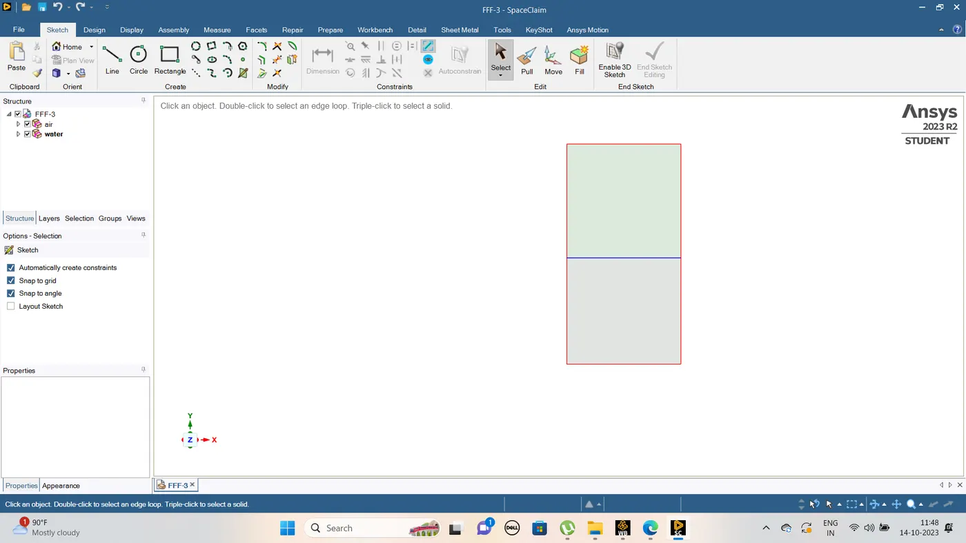
For our project, we consider a simple 2D geometry of which

• We draw 2 squares one above the other with a length of 0.02 m.
• Then naming the below square as air and above square as water in 2 different components.
• And share the topology for a perfect intersection between both surfaces.

STEP 2: MESHING 

CASE 1:

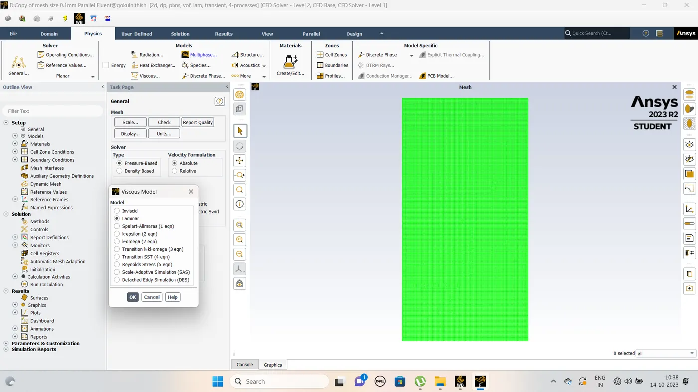
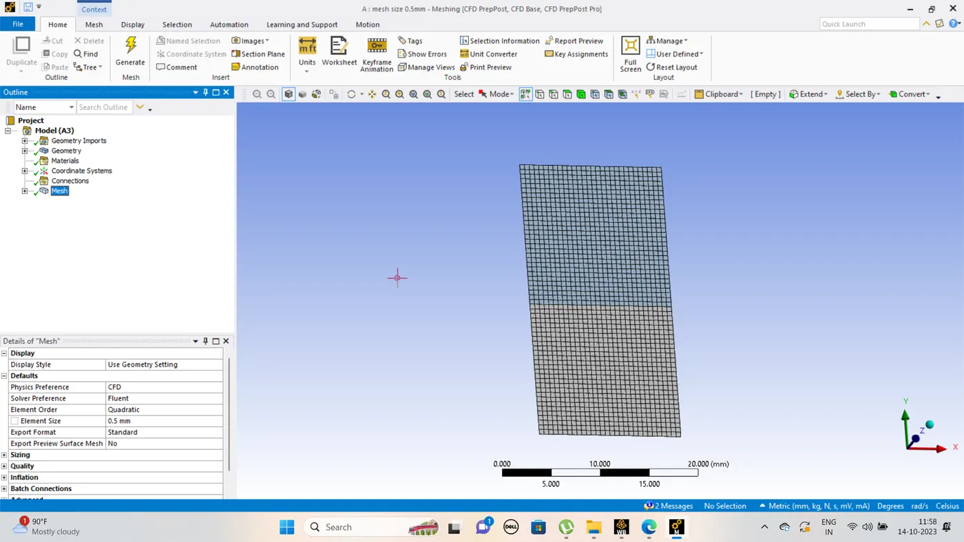
There is not much change to the fundamental mesh as it is a 2D object 

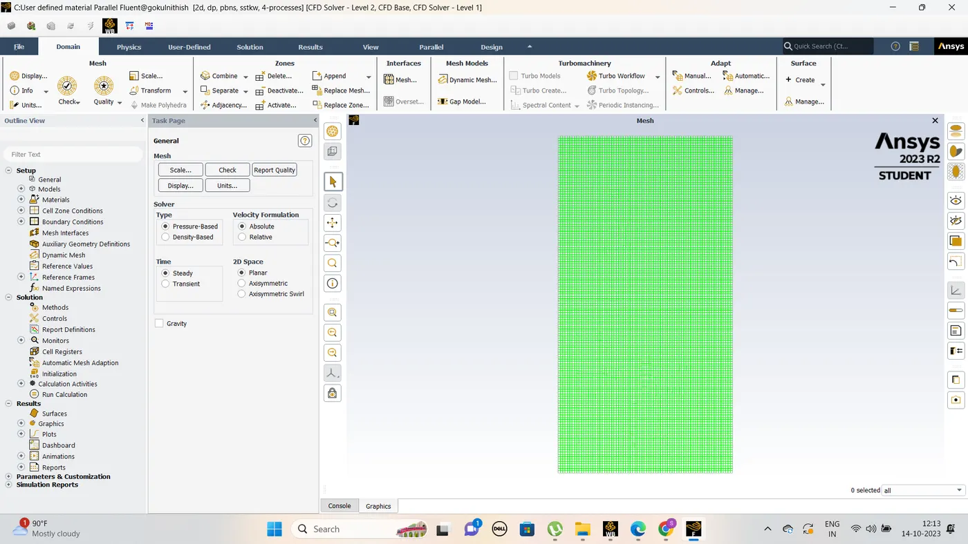
Overall Element size: 0.5mm

STEP 3: SETUP

SETUP
Solver Type	Pressure-Based
Velocity Formulation	Absolute
Time	Un-Steady
Models	Viscous model: laminar Multiphase: Volume of fluid                 : Implicit formulation                  : 2 phases
Material	Fluid type: Air                : water liquid  Solid-type: Aluminium
Cell zones	Fluid type: Air                 : water
Boundaries	Standard
Reference values	Standard
Initialization	Standard Patch: Water-surface (1 value of volume fraction of water)          : Air-surface(0 value of volume fraction of water)

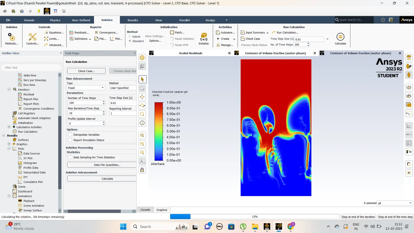
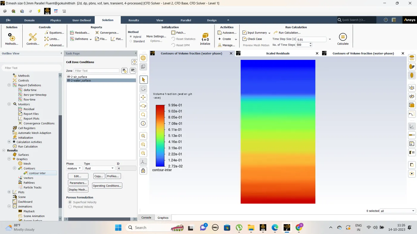
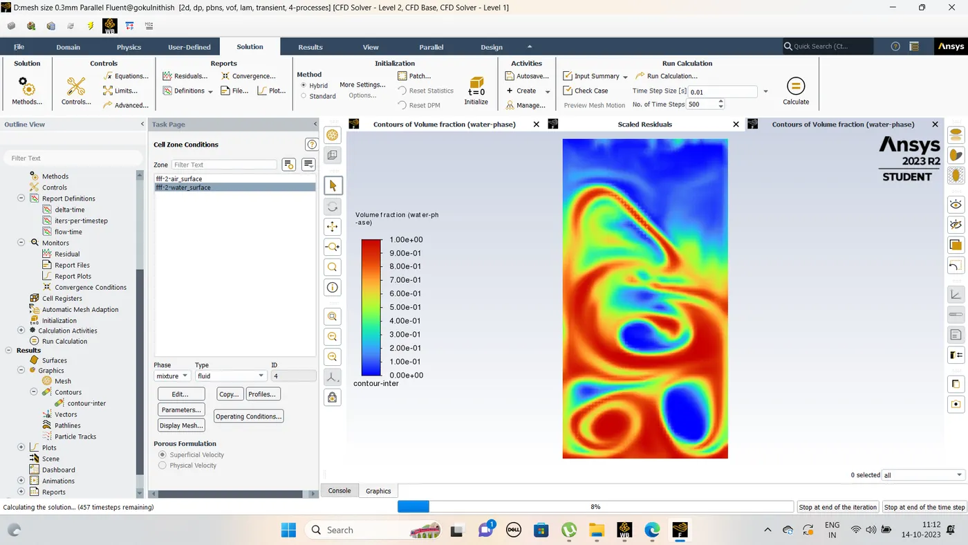
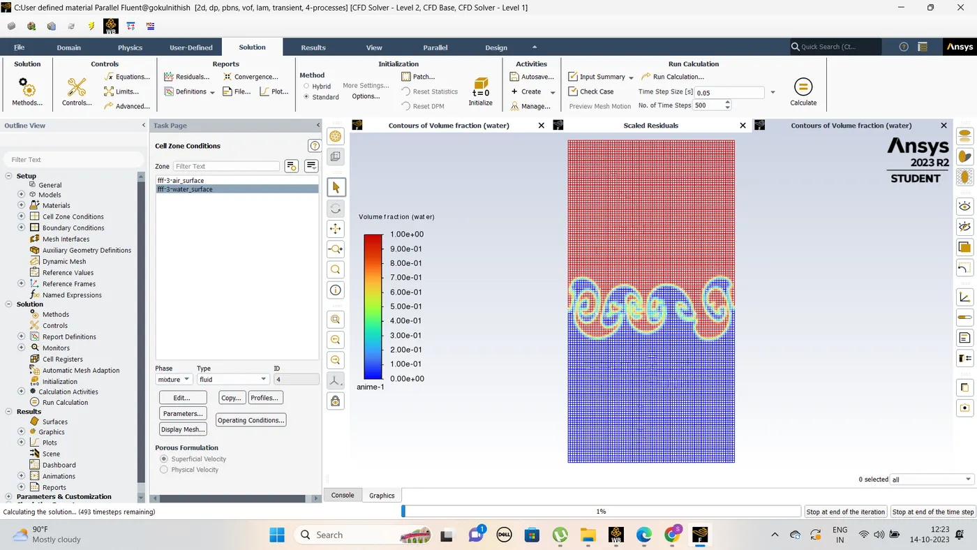
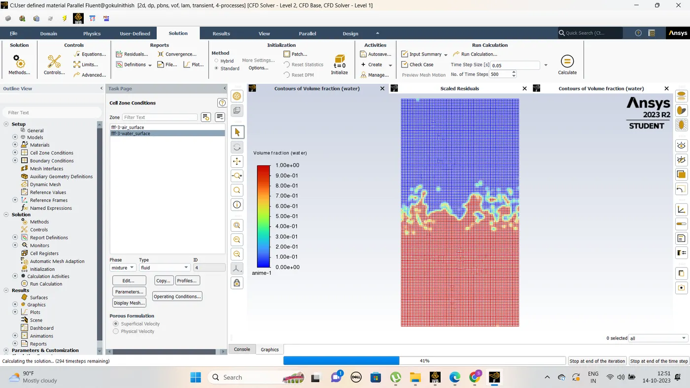
Case 1 : mesh size :0.1mm

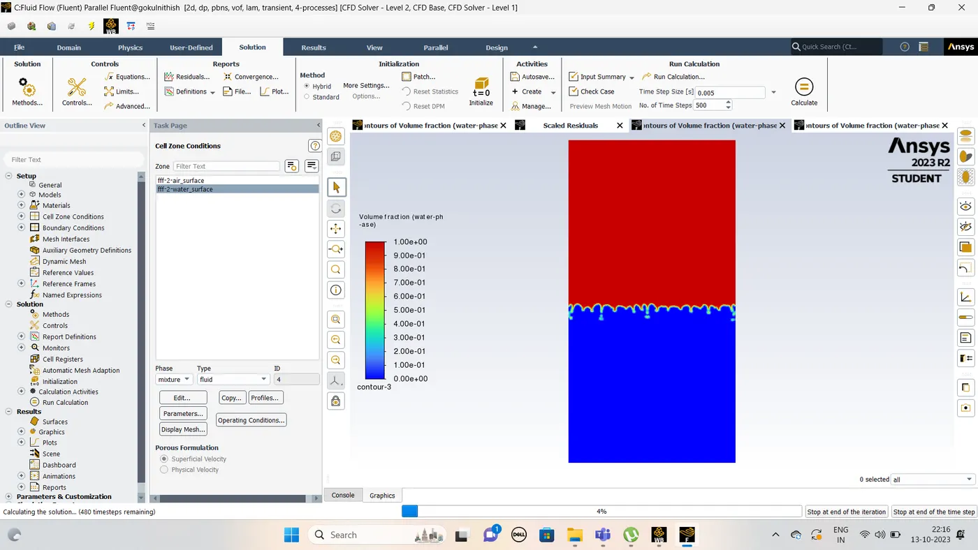
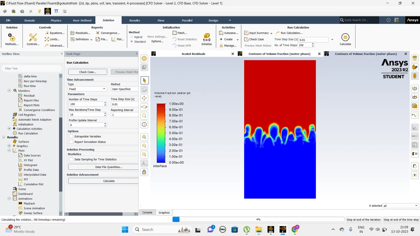
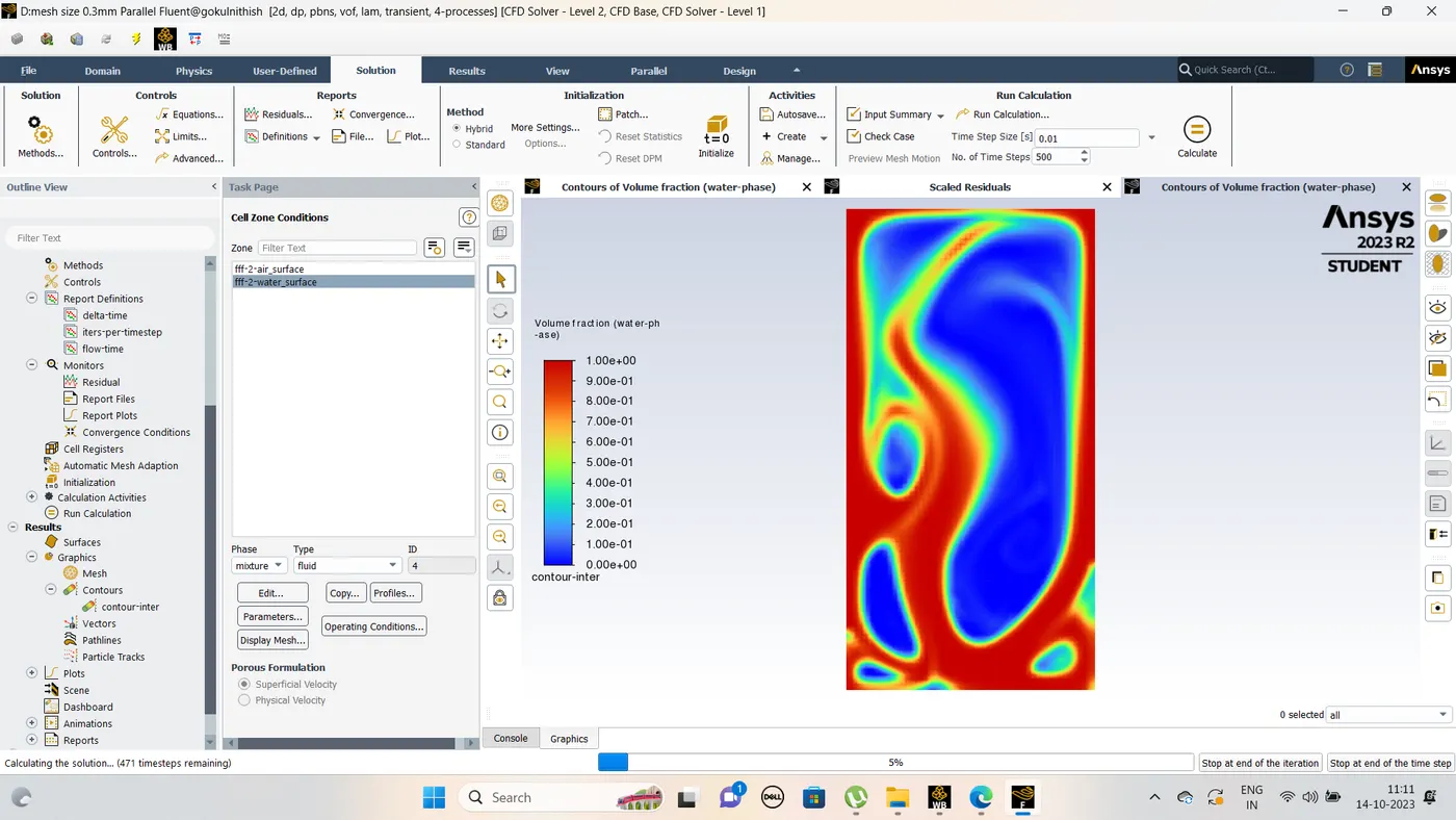
Case 2 : mesh size 0.5mm

Case 3

user defined material refined mesh mesh size 0.2mm

 user-defined material(density = 400 kg/m3, viscosity = 0.001 kg/m-s) for refined mesh. 

STEP 3: SETUP

SETUP
Solver Type	Pressure-Based
Velocity Formulation	Absolute
Time	Un-Steady
Models	Viscous model: laminar Multiphase: Volume of fluid                 : Implicit formulation                  : 2 phases
Material	Fluid type: user define                        material                : water liquid  Solid-type: Aluminium
Cell zones	Fluid type: Air                 : water
Boundaries	Standard
Reference values	Standard
Initialization	Standard Patch: Water-surface (1 value of volume fraction of water)          : Air-surface(0 value of volume fraction of water)

Atwood Number

It is a dimensionless number that is used to study hydrodynamic instabilities in density stratified flows.

Where,

ρ1 is density of heavier fluid 

ρ2 is density of lighter fluid

For Air-water RT instability,

ρ1 = 998.2 kg/m3 [Water density]

ρ2 = 1.225 kg/m3 [Air density]

         A = 0.998

For water- User Defined material RT instability,

ρ1 =  998.2 kg/m3 [Water density]

ρ2 =  400 kg/m3 [UD material density]

        A = 0.428

The behavior of RT Instability on the variation of Atwood number:

RTI evolves in three distinct stages: Linear stability, mushroom head(falling) or bubble(rising) formation, long term evolution due to bubble merging and mixing. For low Atwood number, bubble and mushroom head shape is relatively symmetrical, the disturbances or perturbations are linear for a larger time. In contrast, for large Atwood number, bubble and mushroom head shape is less symmetrical, also it occurs very rapidly at an accelerating rate which leads to a nonlinear growth rate.

CONCLUSION:

• From the above cases, we observe that finer mesh captures the instability better than the coarse mesh, but it takes more time for the heavier fluid to settle down. As computational time is long but produces results with better accuracy.
• Since the simulation involves capturing instabilities that are changing in an unpredictable manner as a function of time, the transient approach is preferred over the steady-state approach. 
• The Atwood no validates the CFD simulation as it is observed. In the case of water and air mixing, bubble formation takes place, whereas in the other case no bubble takes place.