Week 5 - Rayleigh Taylor Instability

CFD Model based on Rayleigh taylor waves:

• Kelvin-Helmholtz instability.
• Richtmyer-Meshkov instability.
• Plateau-Rayleigh instability.

1. Kelvin-Helmholtz instability:

This kind of instability or transition to turbulant flow happens between fluids of different densities moving at different speeds.

in such case a wave formation happens initially this phenomenon is called as Kelvin-Helmholts instability.

As shown in below image.

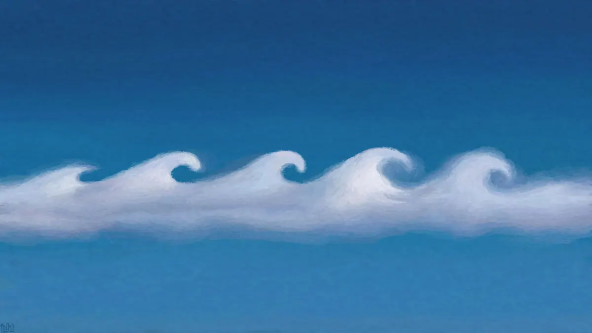
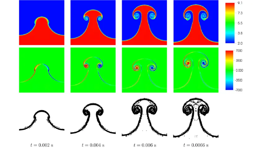
     2.Richtmyer-Meshkov instability:

The Richtmyer–Meshkov instability (RMI) occurs when two fluids of different density are impulsively accelerated. Normally this is by the passage of a shock wave The development of the instability begins with small amplitude perturbations which initially grow linearly with time. This is followed by a nonlinear regime with bubbles appearing in the case of a light fluid penetrating a heavy fluid, and with spikes appearing in the case of a heavy fluid penetrating a light fluid. A chaotic regime eventually is reached and the two fluids mix.

3.Plateau-Rayleigh instability:

It is often called as Rayleigh taylor instability, in which a we understand how a falling stream of fluid breaks up into smaller packets of same volume but lesser surface area.

The driving force of the Plateau–Rayleigh instability is that liquids, by virtue of their surface tensions, tend to minimize their surface area.

Performing simulation on Rayleigh-Taylor instability:

AIM:

To perform a simulation of Rayleigh-Taylor instability concept using two different fluids with different density and viscocity.

Theory:

Rayleigh-Taylor  instability is a concept in which instability happens at interface b/w two different fluids with different densities, lighter fluid pushes heavier fluid. 

Procedure:

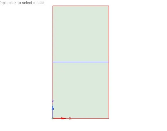
Spaceclaim: Importing of model into space claim and naming to different body/surfaces into air and water.

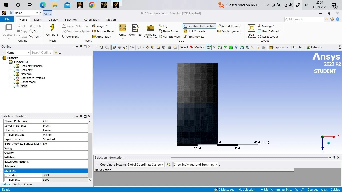
Meshing: Meshing done differently by considering base line mesh(0.5mm) and refined mesh (0.2mm)

Solving: After meshing model is imported to solve in ansys fluent. where all parameters are loaded. which contains, material selection, Phase naming, Patching, animation setup &  contour creation. 

1) Base line mesh (0.5mm)

• Element size: 0.5mm
• No. of nodes: 3321
• No. of elements : 3200.

Material:

water - density = 998.2 kg/m3 , viscosity: 0.001003 kg/m-s

air - density = 1.225 kg/m3, viscosity : 1.7894e-05 kg/m-s

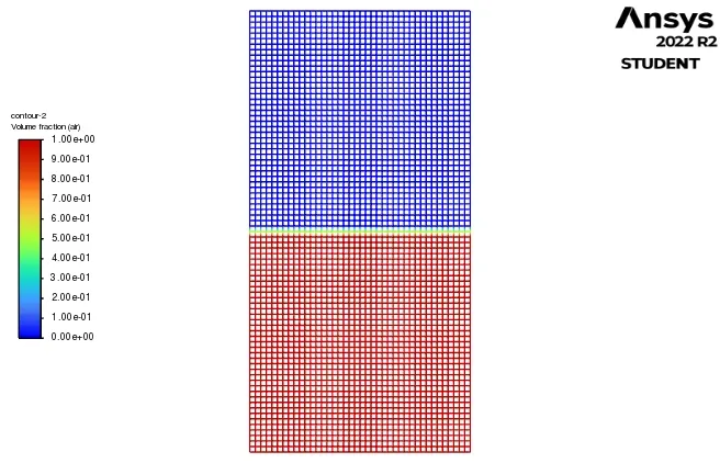
Animation: base line mesh 0.5mm

2) Refined mesh (0.2mm)

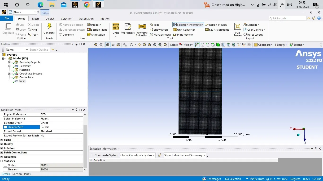
• Element size: 0.2mm
• No. of nodes: 20301
• No. of elements : 20000

Materials

water - density = 998.2 kg/m3 , viscosity: 0.001003 kg/m-s

air - density = 1.225 kg/m3, viscosity : 1.7894e-05 kg/m-s

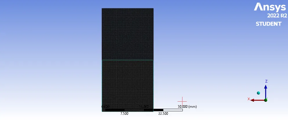
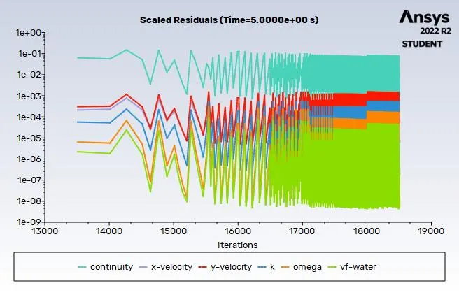
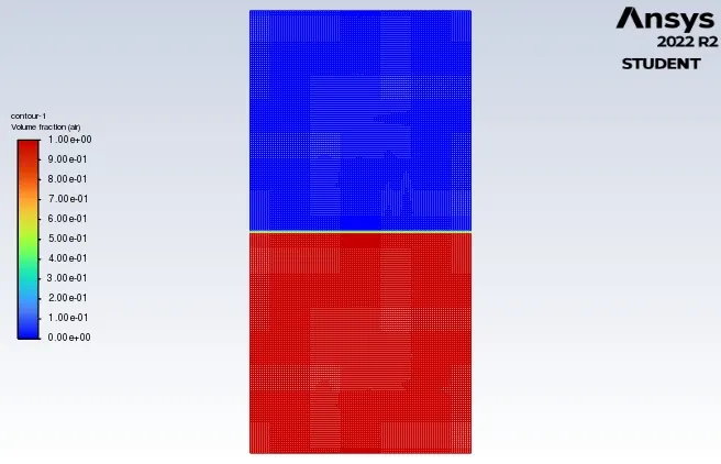
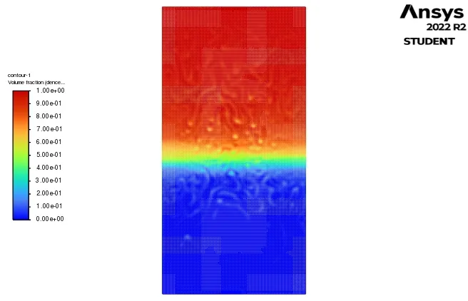
Animation:Refined 0.2mm mesh, air and water.

3) Refined mesh with water and user material:

• Element size: 0.2mm
• No. of nodes: 20301
• No. of elements : 20000

Materials

water - density = 998.2 kg/m3 , viscosity: 0.001003 kg/m-s

user material - density = 400kg/m3, viscosity : 0.001 kg/m-s

Animation: Refined 0.2mm mesh, water and user material

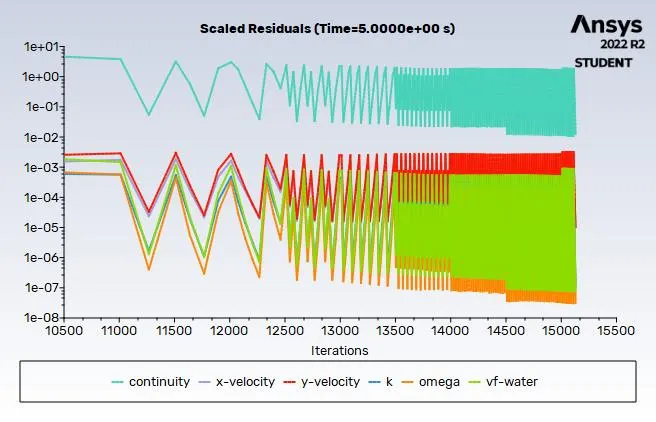
Since its a unsettled phenomenon steady state approach is not suitable.

Atwood number:

The Atwood number is a dimensionless number in fluid dynamics used in the study of hydrodynamic instabilities in density stratified flows. It is a dimensionless density ratio defined as..

A= (rho1-rho2)/(rho1+rho2)

where, rho1 = desnity of heavier fluid

           rho2= density of lighter fluid.

For air and water A= 0.9975

For water and user material A: 0.4278.

 

RESULTS: As the atwood number decreases instabillity increases.

Given model is simulated.

 

 

Animation 1: base line mesh 0.5mm

Animation 2:Refined 0.2mm mesh, air and water.

Animation 3: Refined 0.2mm mesh, water and user material