Week 5 - Rayleigh Taylor Instability
Rayleigh Instability is a hydrodynamic instability that occurs at the interface of two fluids of different densities. Traditionally, the top fluid will be heavier and bottom fluid will be lighter and the gravity will create the instability between the two which leads to mixing and interpenetration of the fluids. This instability model is used in fields of astrophysics, engineering and fluid dynamics.
Some practical examples:
1) Nuclear bomb testing: In the past, during nuclear testing, the detonation created huge shockwaves which leads to Rayleigh instability between the interfaces of the fireball and the surrounding air. This study helped researcher refine the models for nuclear explosion.
2) Wildfire Spread: In wildfire, Rayleigh instability can be observed between hot air above the flames and cold denser air below. This instability leads to generation of fire clouds which then affects weather pattern, fire behaviour etc.
For Rayleigh Instability we will be running 3 cases
1) Case 1: Observing Instability Animation with a base mesh of 0.5mm between water and air interface
2) Case 2: Observing instability animation with a refined mesh of 0.2mm between water and air
3) Case 3: Observing Instability animation with refined mesh between user defined fluid and water
Pre-Processing
1) First, we will create 2 square boxes of size 20mm X 20mm which will represent the initial stage of water and air at top and bottom respectively.
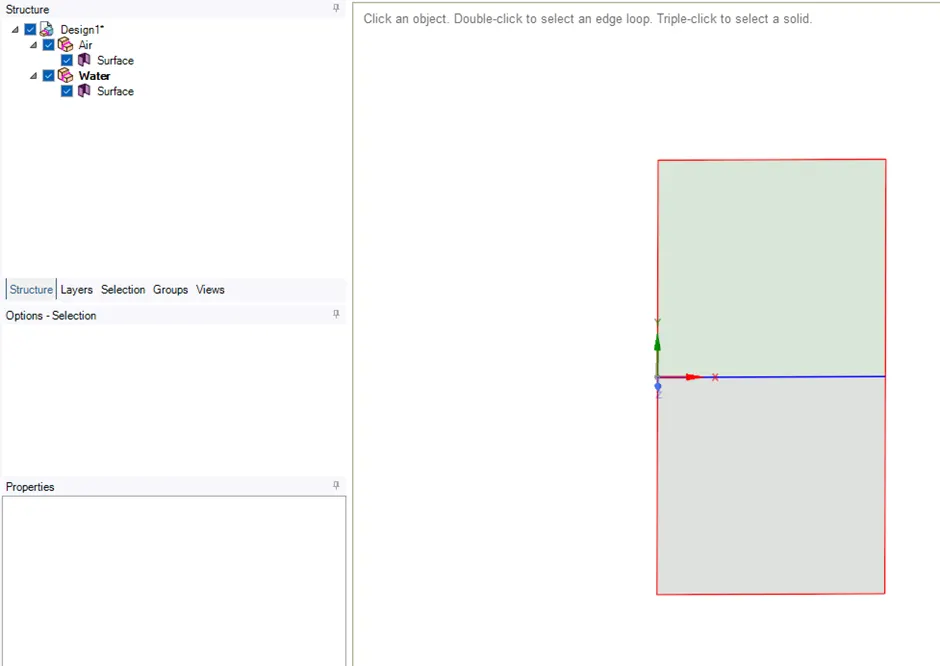
Now, we will move forward with Case 1 and Case 2
CASE 1
Meshing
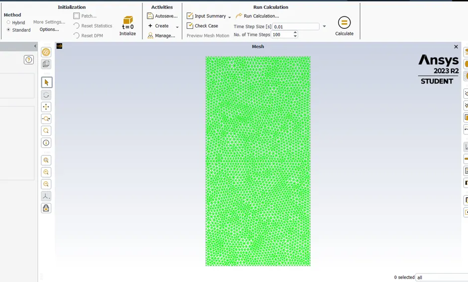
The Mesh is as shown in below:
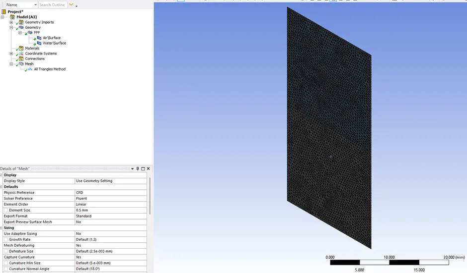
Mesh size in 0.5 mm.
SETUP:
We will be using pressure-based solver with transient state. We will also take gravity into account for this simulation.
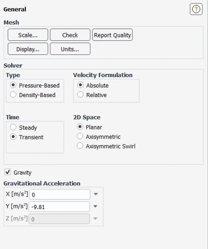
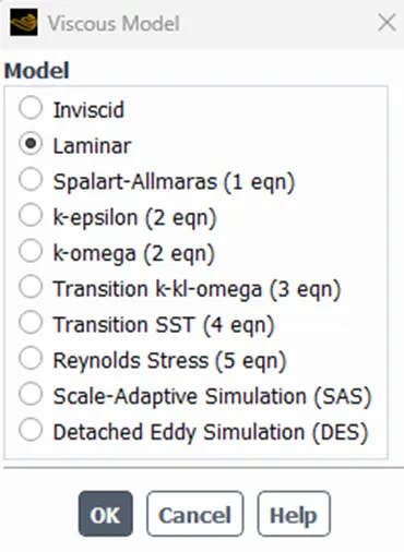
Materials used are air and water
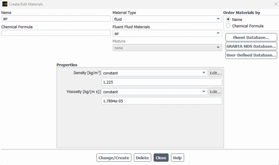
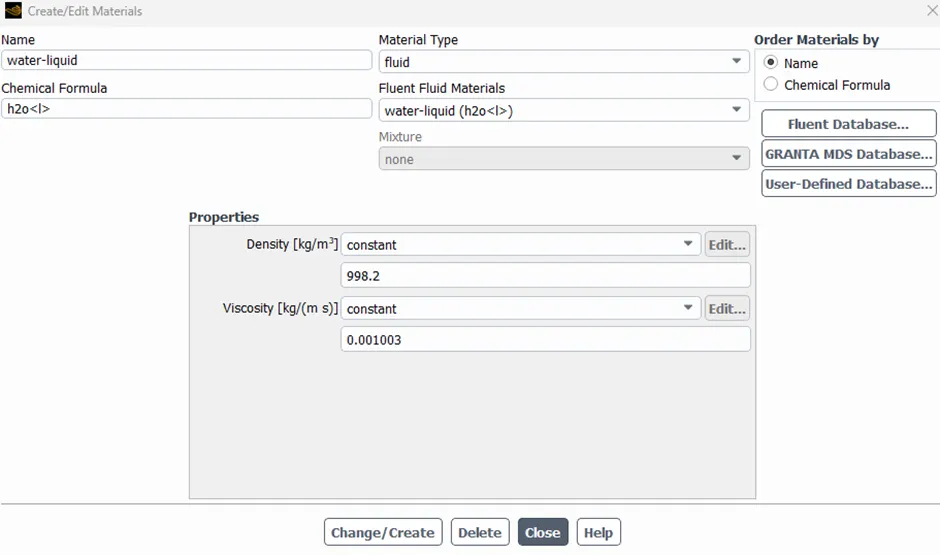
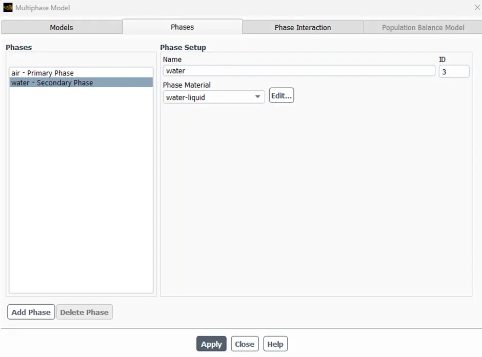
We will use Volume of Fluid model with 2 Eulerian phases
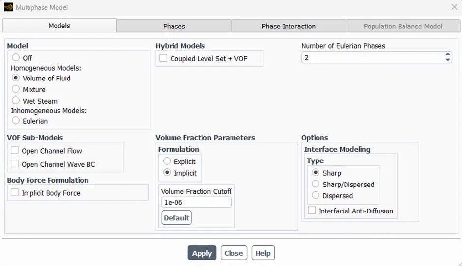
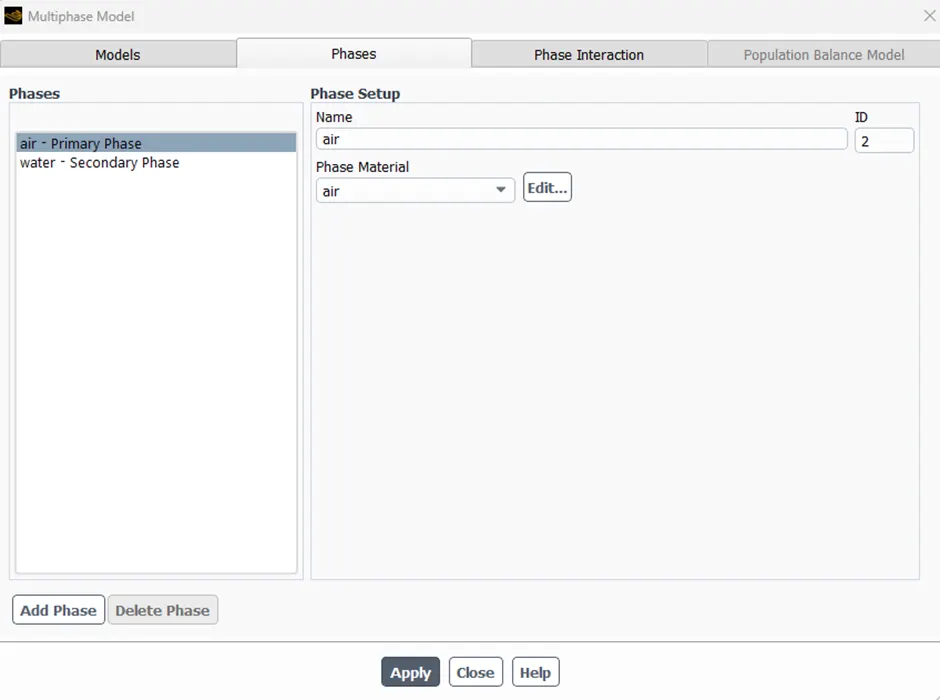
Once setup is done, we will initialize the model with standard approach and then patch the phases to the model.
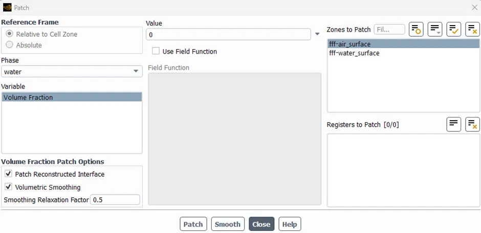
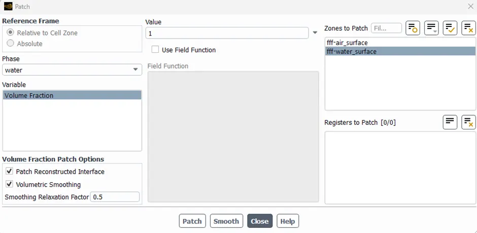
We can confirm the proper patch of the model by viewing contours
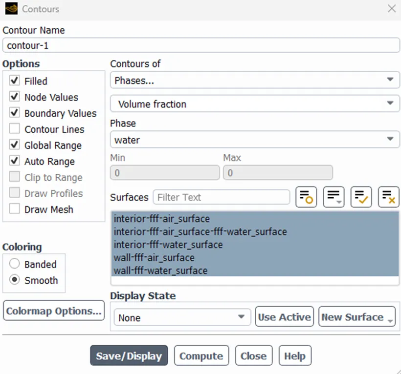
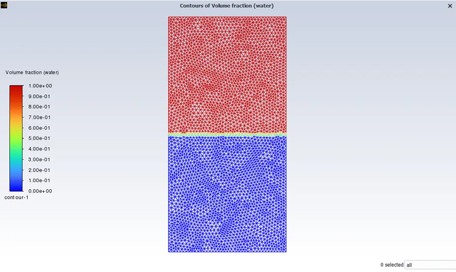
We will set time step size to 0.005 and No. of time steps to 100 and will begin calculation.
Also, we will setup the solution animation for the same.
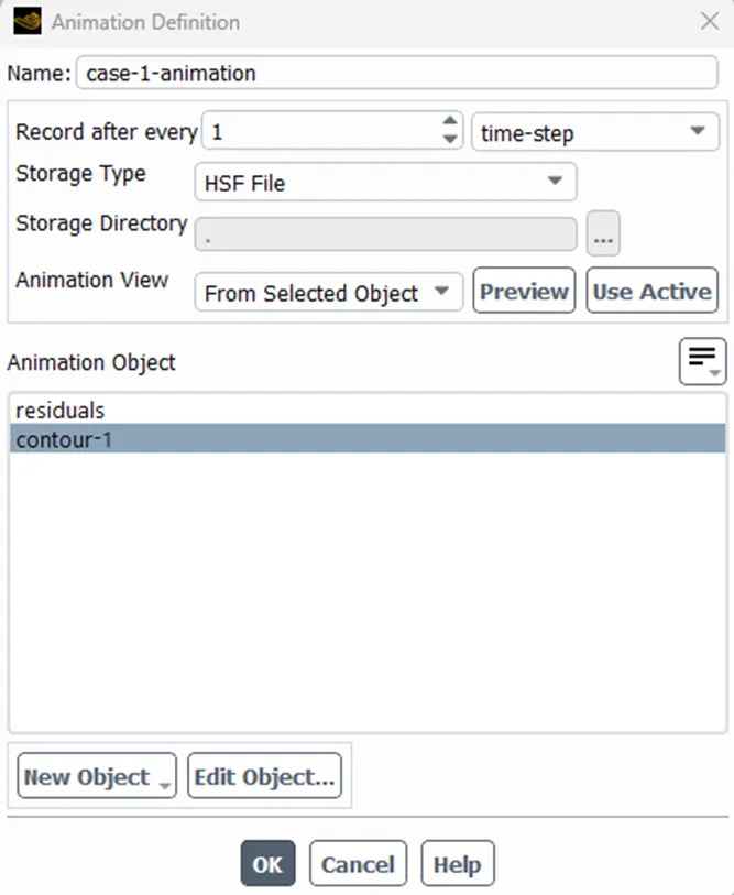
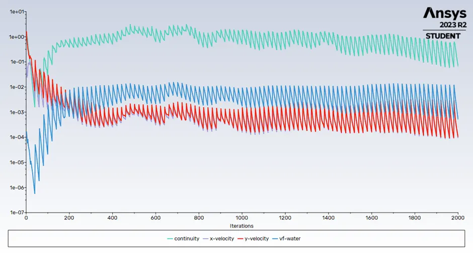
Residual Chart
Animation is in the attachments
CASE 2
MESHING
Mesh is as shown below
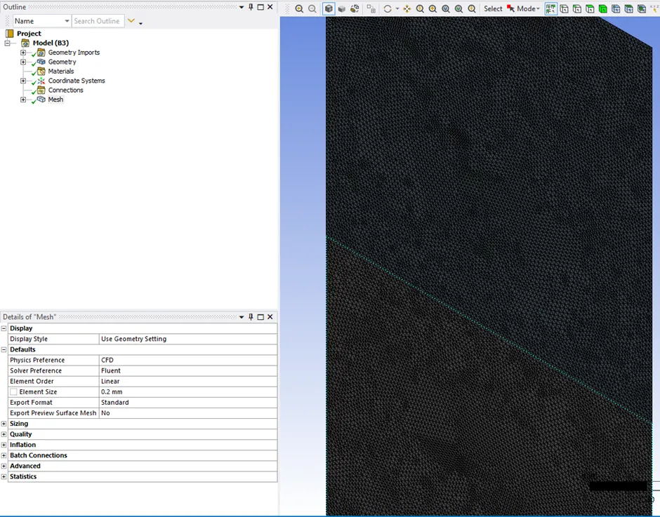
Mesh size in 0.2 mm
Setup
Setup will be same as in case 1.
Residual Chart
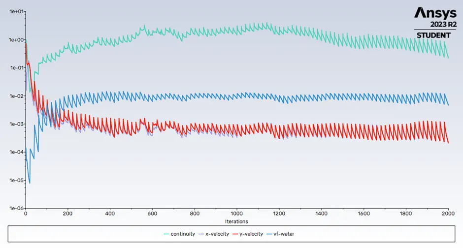
Please look at the animations provided in the attachment
CASE 3
Pre-Processing
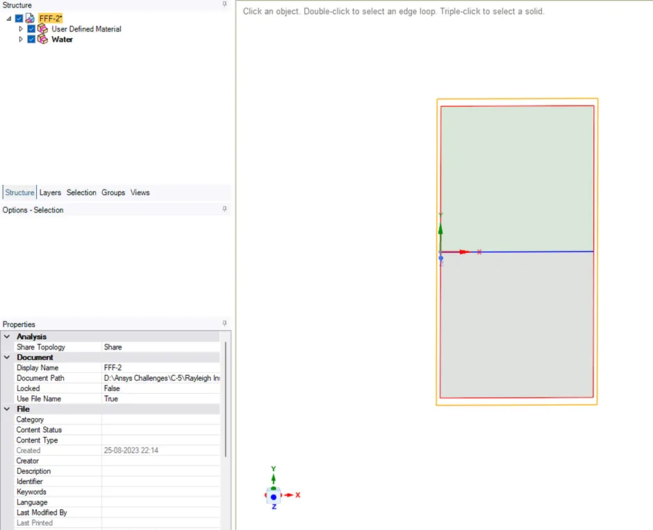
MESHING
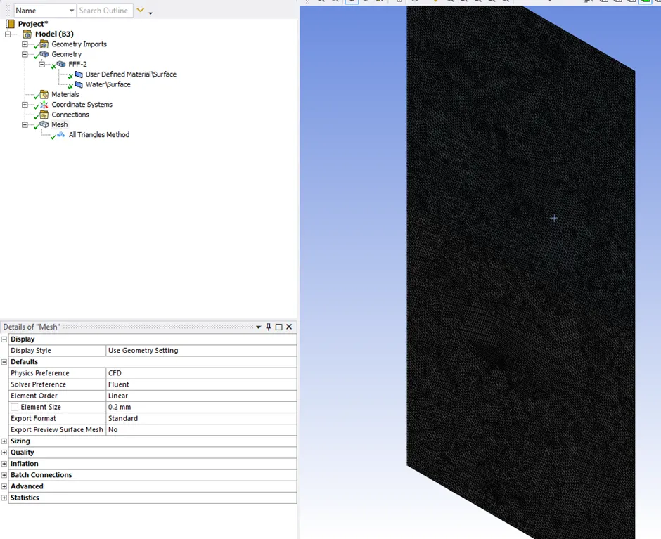
In Case 3, we will have the same meshing as case 2.
SETUP
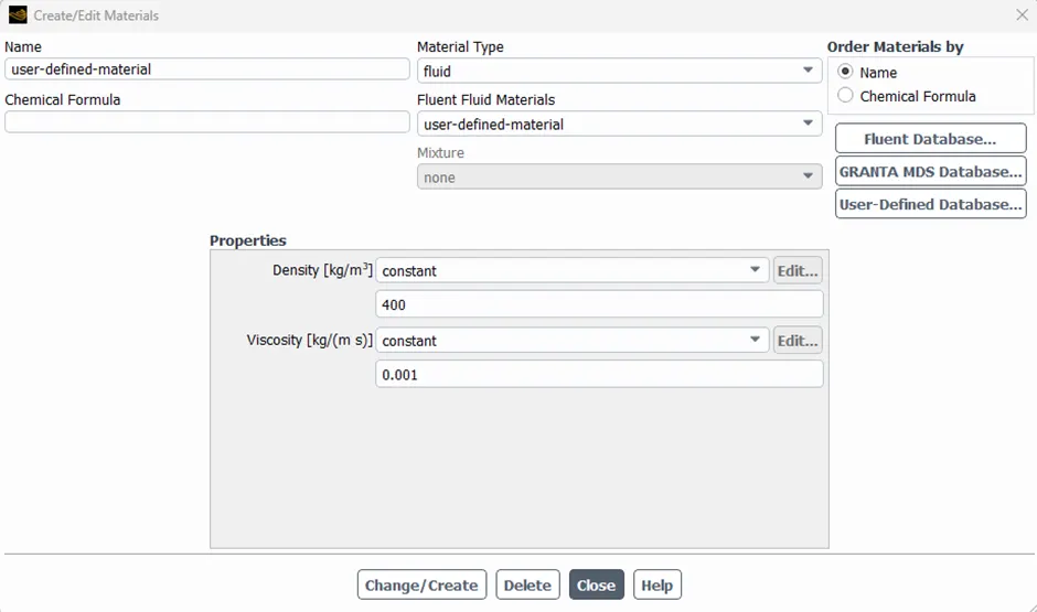
In Case 3, we are replacing air with a user defined material. The properties of the same material is as below
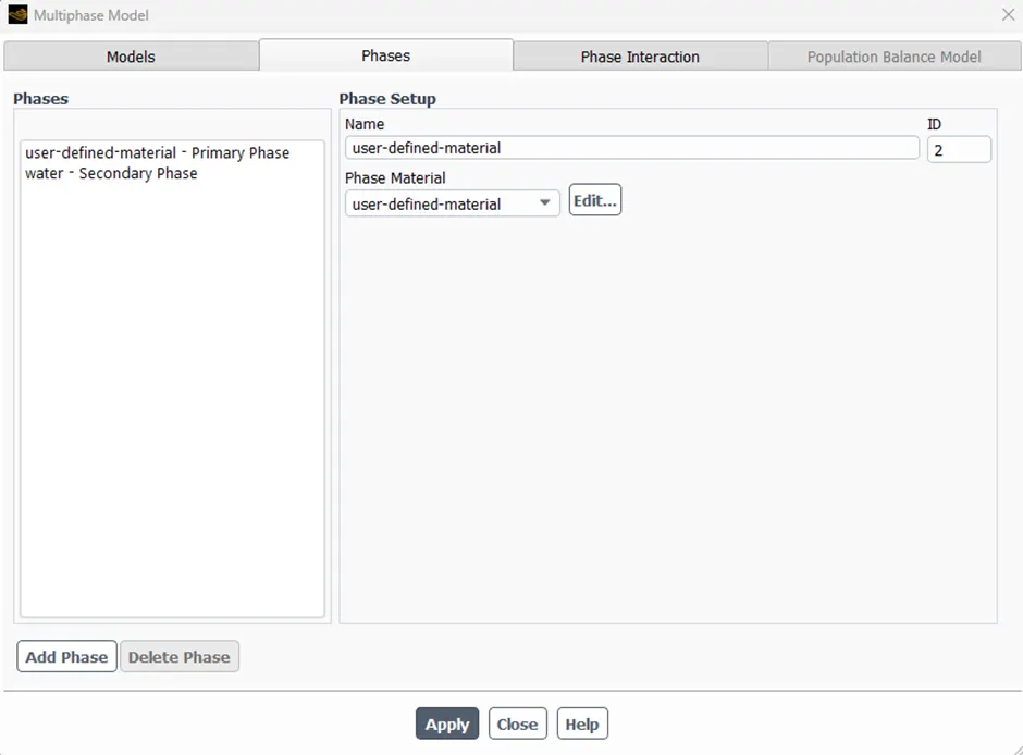
Now we will update the phase accordingly
After initializing the solution, we will patch the phases to the model.
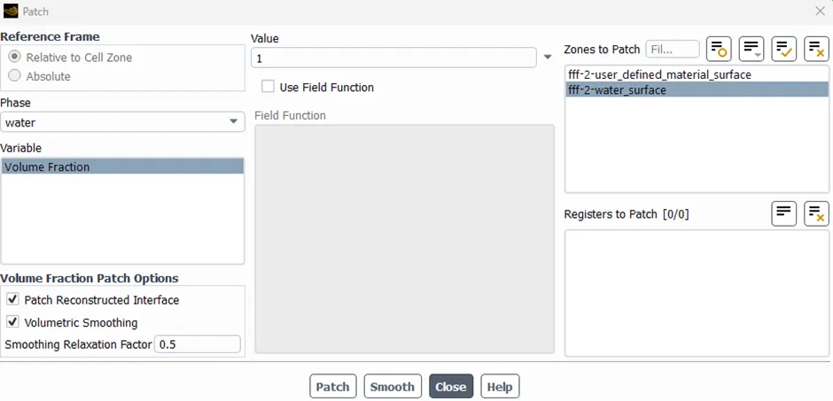
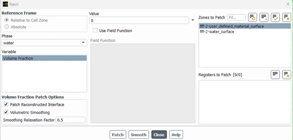
We can confirm the patch by viewing the contour
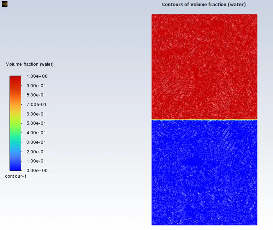
We will set time step size to 0.005 and No. of time steps to 100 and will begin calculation.
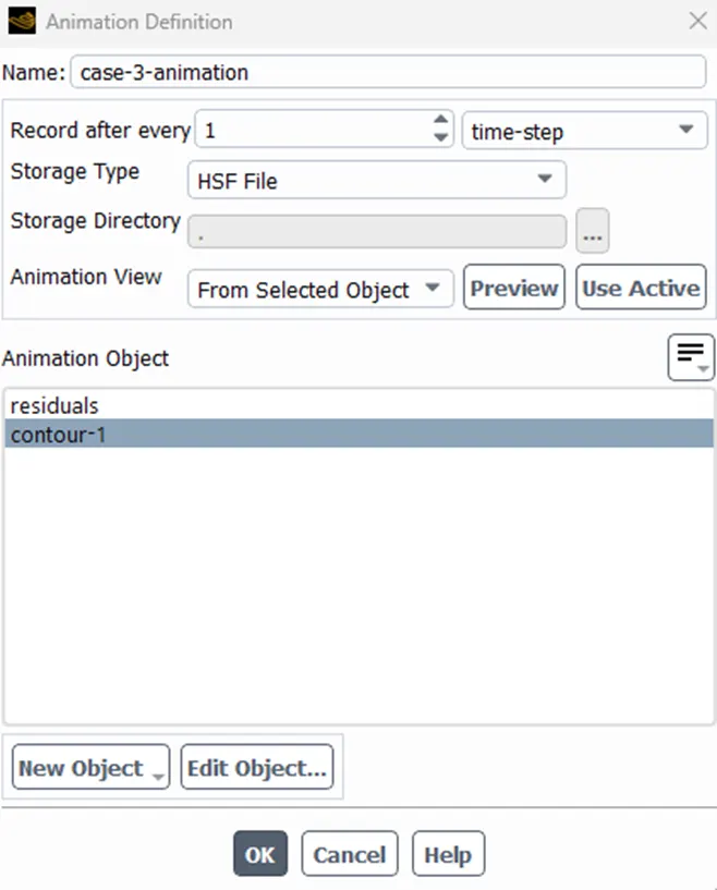
Also, we will setup the solution animation for the same.
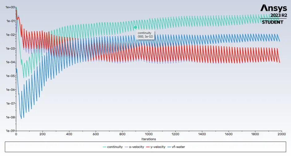
Residual Chart
Please look at the animation provided in the attachment
CONCLUSIONS:
1) With a refined mesh we can see that the instability is captured better than the coarser mesh.
2) The result obtained have better accuracy but the computational time increased
3) We use Transient solver rather than steady state solver because we needed to know how the mixing take place in real time rather than the end results. When only end result is of concern then we use steady state solver, but for real time simulation we will use transient solver.
ATWOOD NUMBER
Atwood Number is a dimensionless quantity used in fluid dynamics to characterize the fluid in gravitational field.
At = (ρ1 - ρ2) / (ρ1 + ρ2)
Where,
ρ1 = density of heavier fluid
ρ2 = Density of light fluid
Here in case 1 and 2 we have,
ρ1 = 998.2 kg/m3 (Water)
ρ2 = 1.225 kg/m3 (Air)
So, we get At = 0.9975
In Case 3,
ρ1 = 998.2 kg/m3 (Water)
ρ2 = 400 kg/m3 (User defined material)
So, we get At = 0.4278
Fluids with Atwood number close to 1 have major difference in their density, which results in larger bubble. The flow is very rapid
Fluids with Atwood number close to 0 have very less difference in their density, which forms symmetrical bubbles. The flow is comparatively slow and linear.