Week 1- Mixing Tee
Aim: To perform a Fluid flow analysis of a Mixing Tee component using hot and cold air through 2 inlets. We will define the relation between the length of the mixing tee component and the temperature of the air at the outlet. Also, the variation in the outlet temperature based on the velocity of cold Air. We will also perform a mesh sensitivity run to check if the result differs based on change in mesh length.
For this analysis, In ansys workbench i have selected Fluid Flow workbench
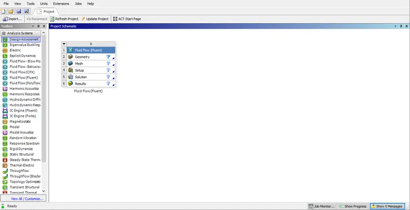
Pre-Processing and setting up Boundary Condition:
a) we will first import the step file for the mixing tee provided in spaceclaim. here we have to define a wet volume as it will represent the fluid flow inside the mixing tee. We can use volume extract option to define the volume inside mixing tee.
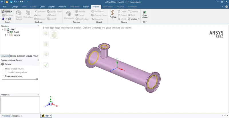
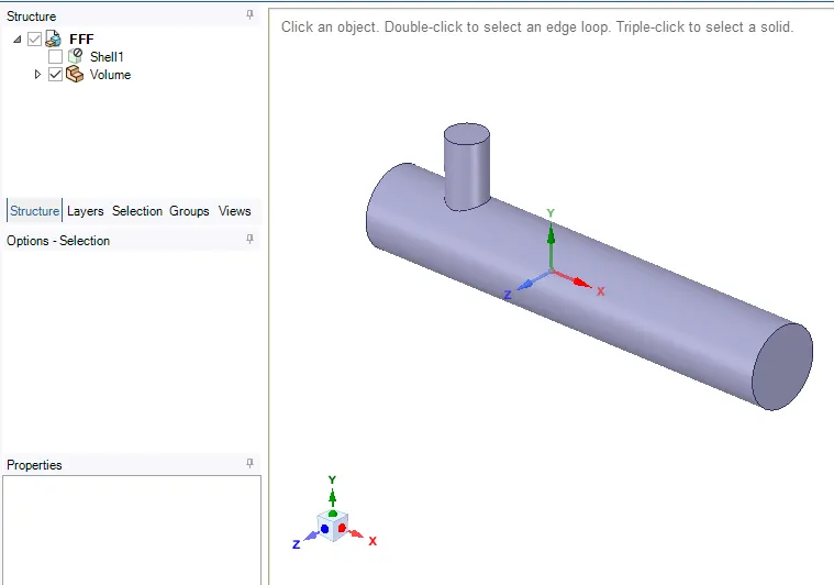
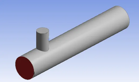
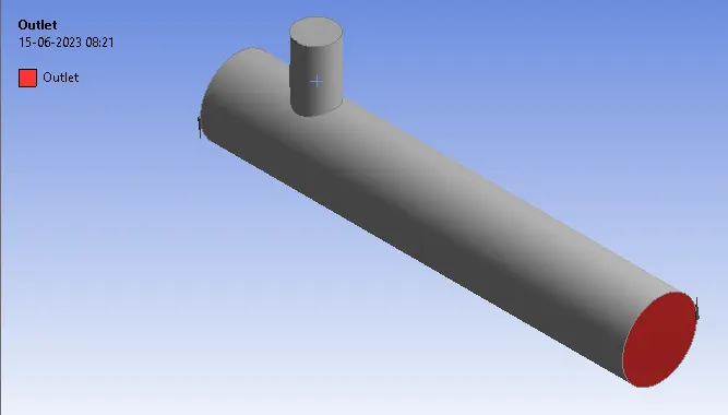
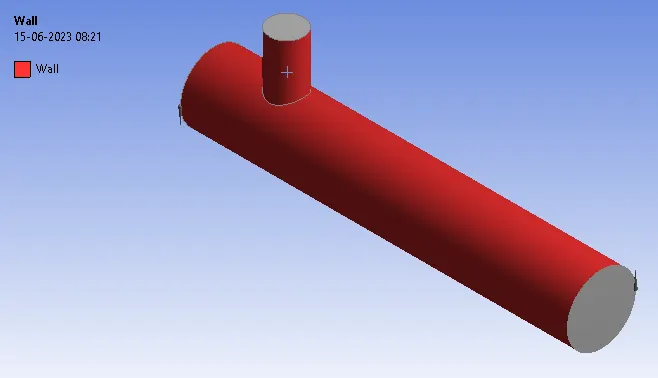
b) Once volume is extracted we move to meshing workbench, here first we assign names to the faces for proper defining of boundary conditions in later stage. Below are the images for the same.
Cold air inlet:
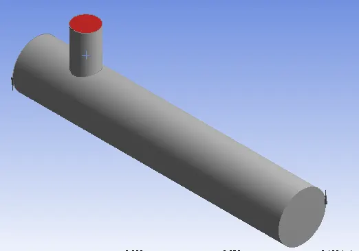
Hot air inlet:
Outlet:
Wall:
c) Once the faces are named then we move onto meshing the model. By setting mesh parameters we can generate mesh in the workbench.
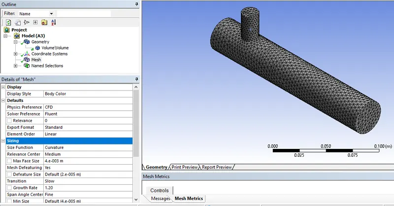
Mesh quality is displayed in the Case specific sections.
d) once mesh is defined we move on with setting up the boundary conditions. to setup boundary condition we move to fluent workbench.
- Once the fluent workbench is open, we can start with checking the mesh to confirm there are no errors.
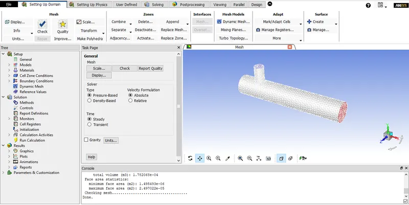
- Now we can move forward with the setting up of physics for solving along with the boundary condition. So, for this solving we have selected steady state solving with pressure based type and velocity formulation to absolute. As we need temperature as an output we have selected energy and will be using viscous model with K-epsilon realizable and K-omega for our first case.
- After this we can setup boundary condition.
- For Hot air inlet:
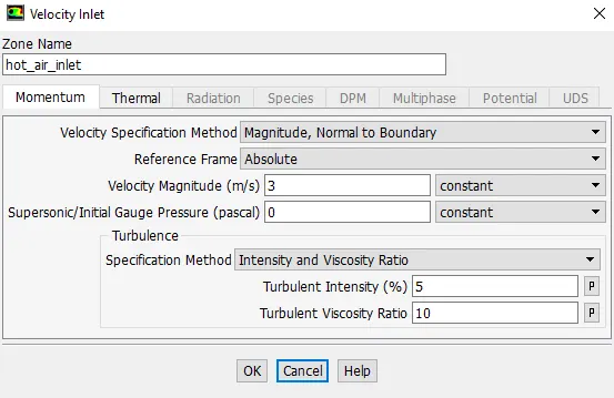
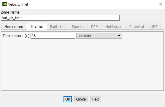
- For cold air inlet the inputs will change as per the cases we are solving
- For outlet gauge pressure is set to zero.
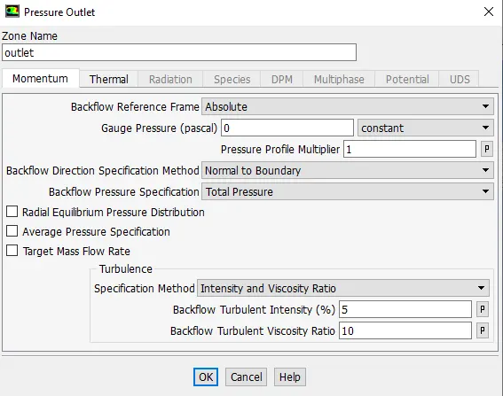
- For Hot air inlet:
Case Studies and Results:
1) K-epsilon Model V/s K-omega Model:
Aim: To determine the type of Viscous model to move forward with for other case studies.
Type of Model: Long Pipe
No. of Iterations: 350
Cold Air inlet Velocity and Temperature: 12 m/s and 19 Deg Celsius
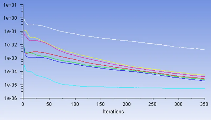
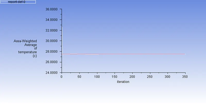
a) Type of Viscous Model: K-Epsilon Realizable
Result:
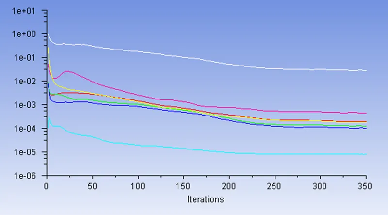
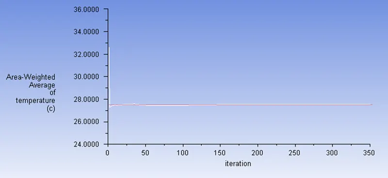
b) Type of Viscous Model: K-Omega SST
Result:
Conclusion:
When comparing K-epsilon model and K-omega model we don't see much difference in the average temperature we get i.e approx 27.5 Deg Celsius. But if we look at the convergence for K-epsilon Realizable the convergence looks better than the K-omega.
So, for upcoming cases K-epsilon Realizable model will be preferred.
2) Mesh Independency test:
a) Mesh Length - 4mm
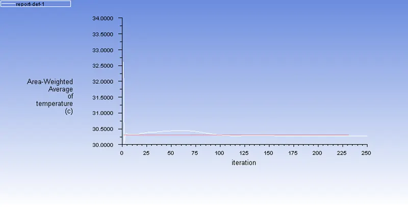
At mesh length of 4 mm we are getting temperature around 30.3 deg Celsius.
b) Mesh Length - 1mm
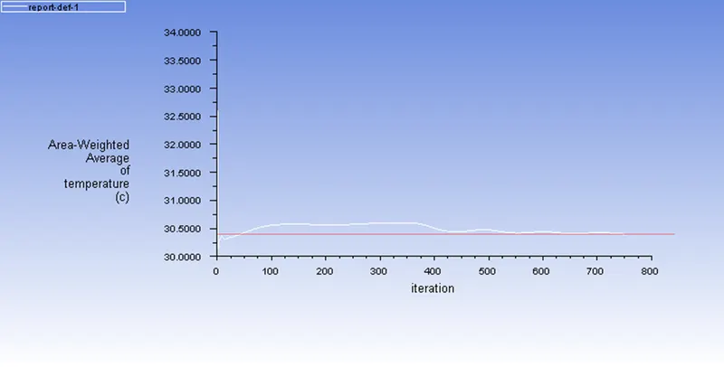
At mesh length of 1mm we are getting a temparature of around 30.4 deg Celsius.
So, as there is not much variation in the result we can opt for 4mm mesh length for further analysis.
3) Case 1:
Type of Model: Short Pipe
Momentum Ratio: 2
Velocity of cold air: 6m/s
Mesh length: 4mm
Cell count: 22116
No. of Iterations: 350
Avg. Temp: 30.3 C
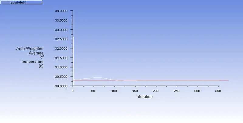
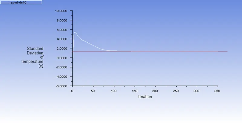
Standard Deviation: 1.2 deg C
Temperature and Velocity Plotting across the pipe:
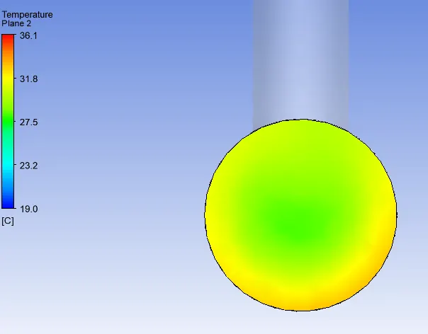
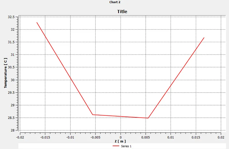
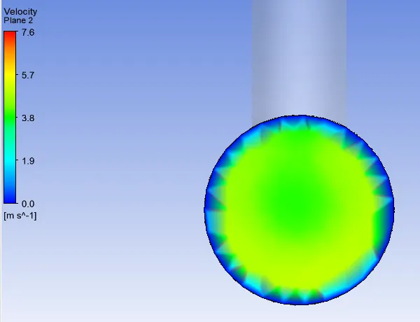
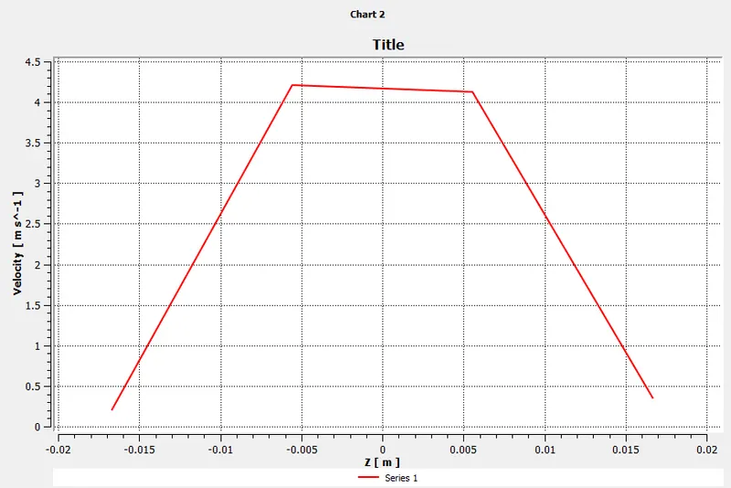
Temperature and Velocity Plotting along the pipe:
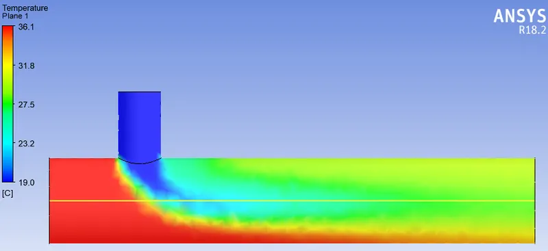
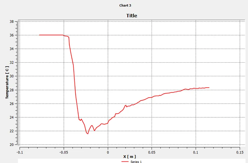
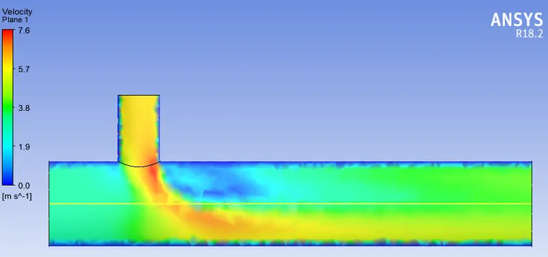
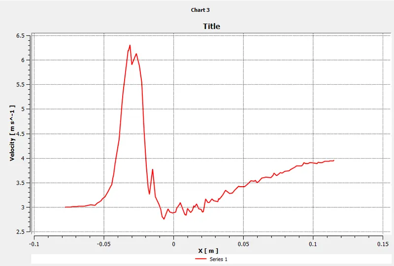
4) Case 2:
Type of Model: Short Pipe
Momentum Ratio: 4
Velocity of cold air: 12m/s
Mesh length: 4mm
Cell count: 22116
No. of iterations: 350
Avg temperature: 27.5 deg C
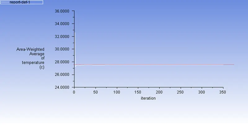
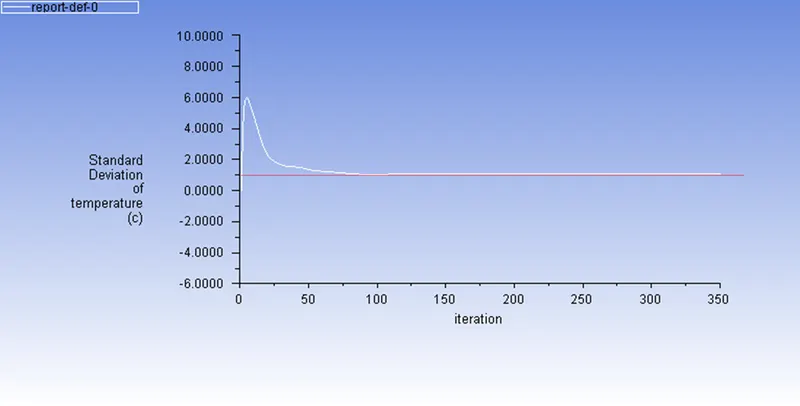
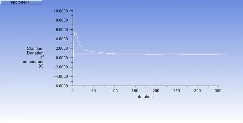
Standard Deviation: 1 deg C
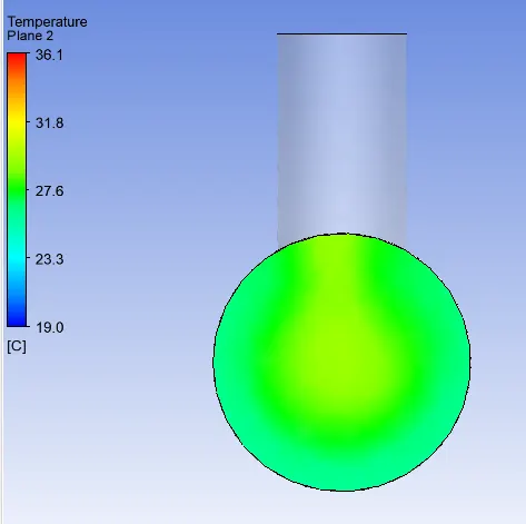
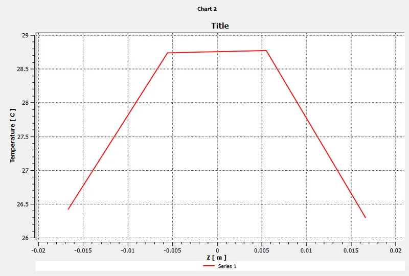
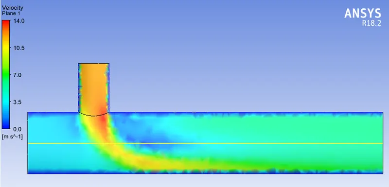
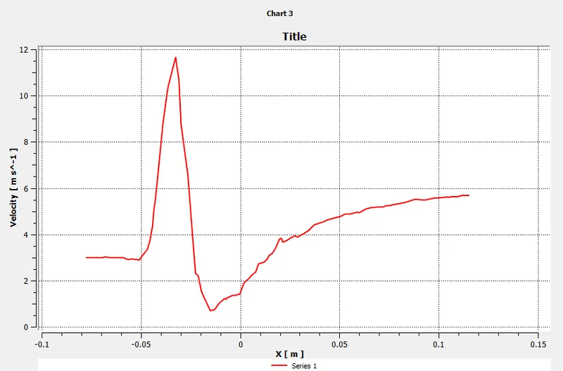
Temperature and Velocity Plotting across the pipe:
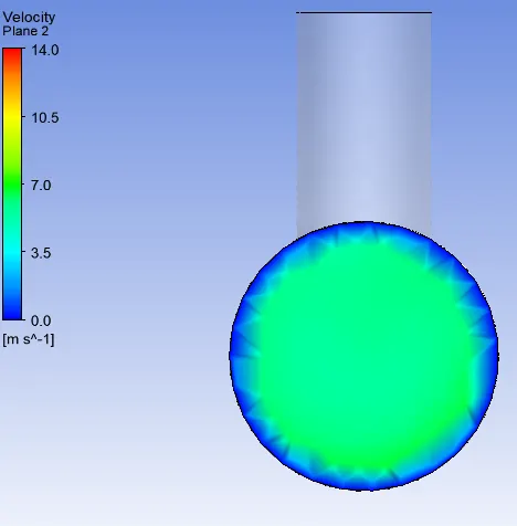
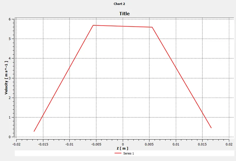
Temperature and Velocity plotting along the pipe:
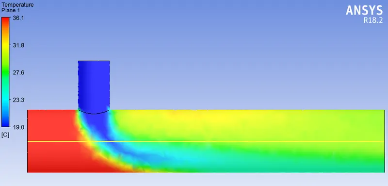
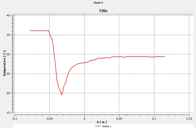
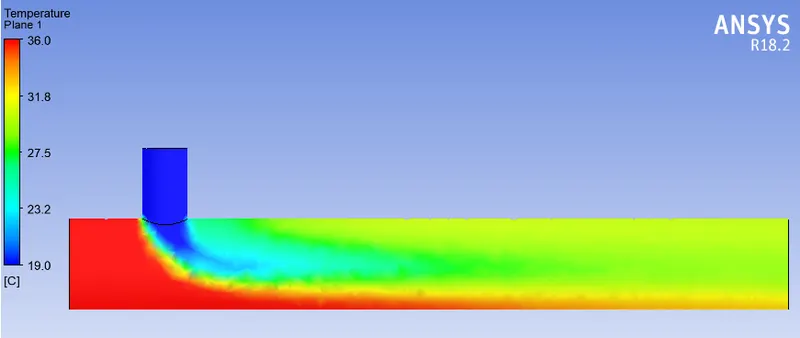
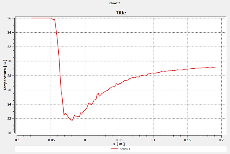
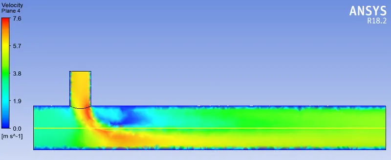
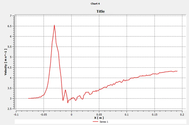
5) Case 3:
Type of Model: Long Pipe
Momentum Ratio: 2
Velocity of cold air: 6m/s
Mesh length: 4mm
Cell count: 28907
No. of iterations: 350
Avg temperature: 30.3 deg C
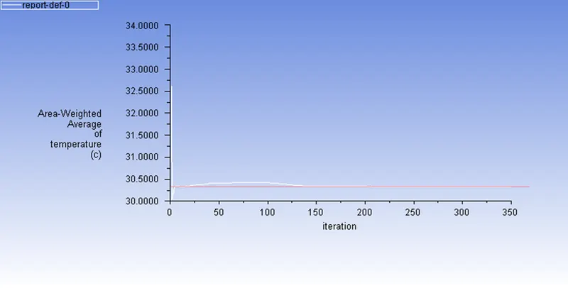
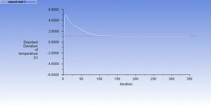
Standard Deviation: 1 deg C
Temperature and Velocity Plotting across the pipe:
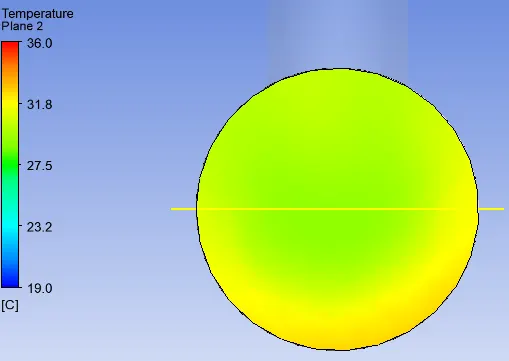
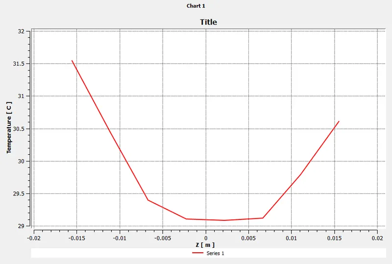
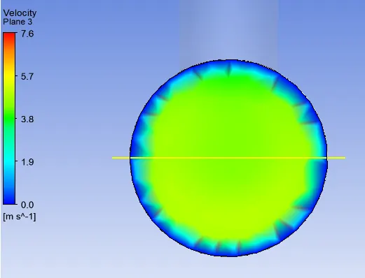
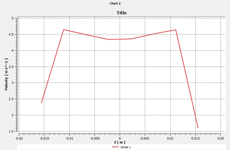
Temperature and Velocity plotting along the pipe:
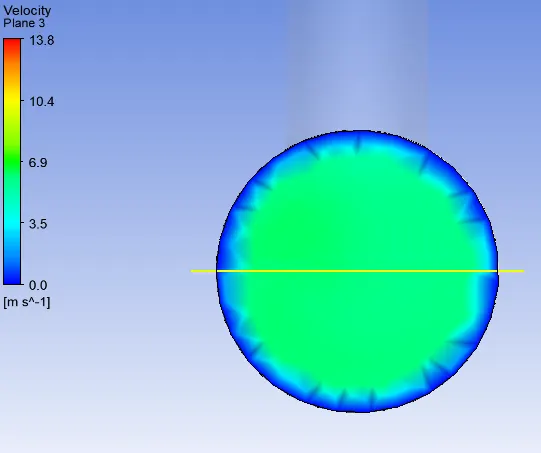
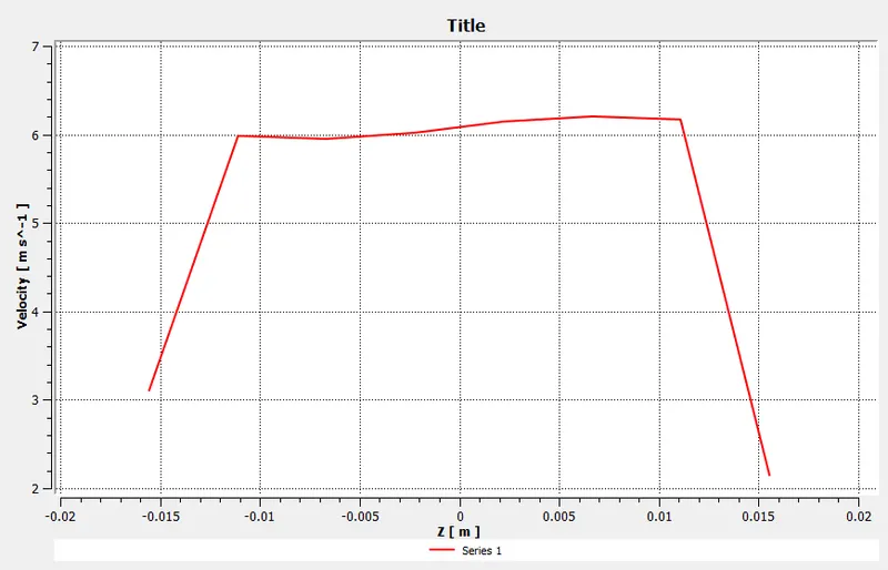
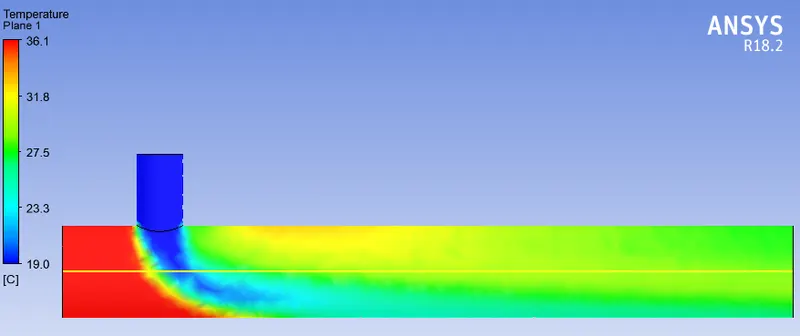
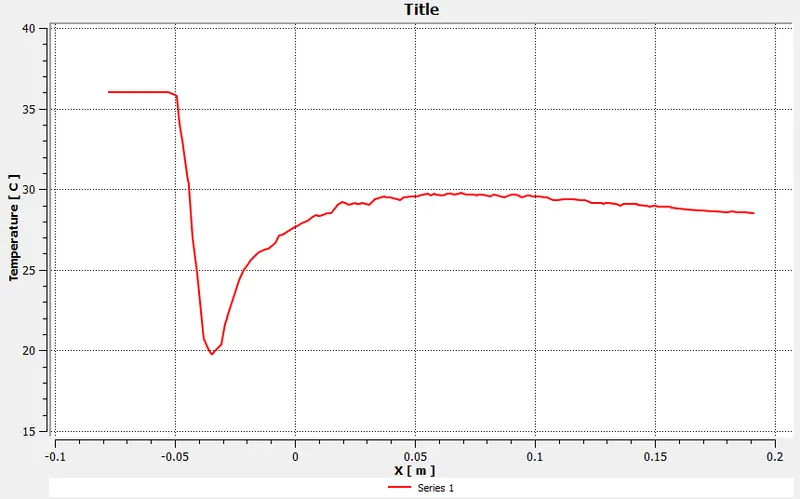
5) Case 4:
Type of Model: Long Pipe
Momentum Ratio: 4
Velocity of cold air: 12m/s
Mesh length: 4mm
Cell count: 28907
No. of iterations: 350
Avg temperature: 27.5 deg C
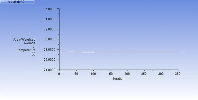
Standard Deviation: 0.9 deg C
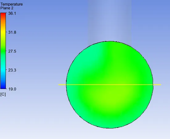
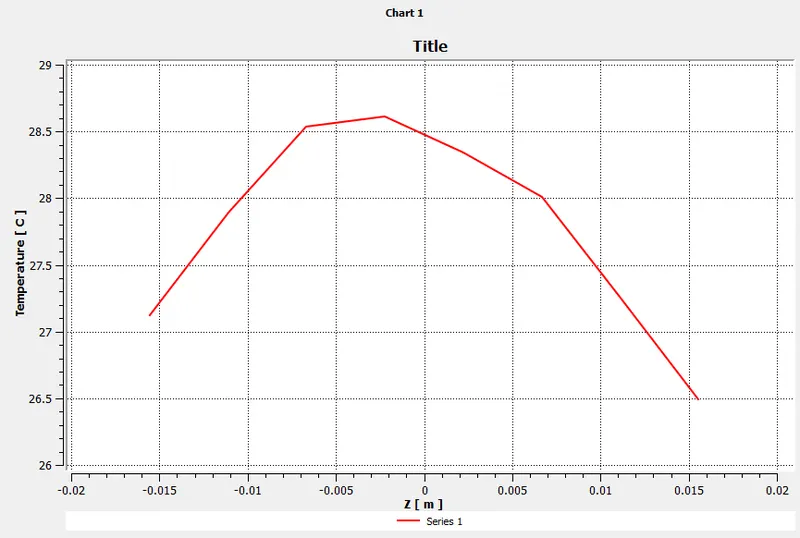
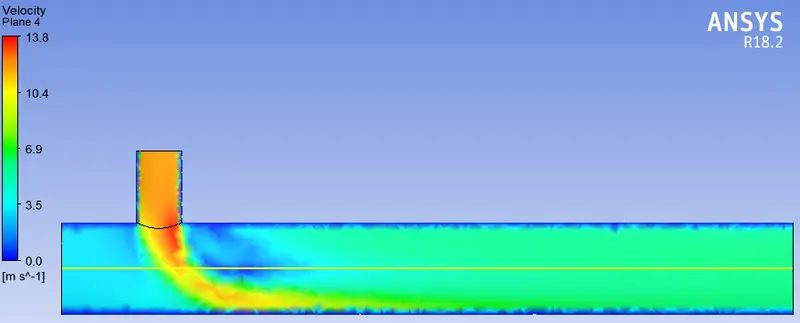
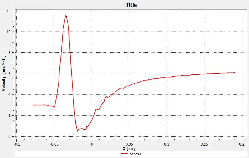
Temperature and Velocity Plotting across the pipe:
Temperature and Velocity Plotting along the pipe:
Results:
Comparison Based on length of the pipe:
When we compare the result based on length of the pipe we see that there is almost not change in the weigted average temperature at the end of the pipe. But when you observe the temperature graph across the pipe and also the standard deviation for Long pipe and Short Pipe, we can say that the mixing of Cold and Hot air is better in Long pipe than in Short pipe.
with this we can conclude that as the length increases the mixing increases as well.
Comparison Based on Velocity of Cold Air:
When we compare the result based on the velocity of cold air we can see that the drop in temperature is noticable from around 30 deg C to 27 deg C approx. So, because of increase in velocity the temperature drop is noticable. We can also make an observation that the mixing of air is better with increase in the velocity of cold air, as standard deviation for the temp decreases. Net velocity of the air also increases with increase in velocity of cold air
With this we can conclude, with increase in velocity of cold air, Avg temperature decreases, Mixing increases and Velocity increases as well