Week 5 - Rayleigh Taylor Instability

WEEK 5: RAYLEIGH – TAYLOR INSTABILITY

AIM

The challenge comprises of grid independence study performed to understand the Rayleigh – Taylor instability in Ansys Fluent and effect on R-T instability due to variation in Atwood number.

INTRODUCTION

Rayleigh – Taylor Instability:

The Rayleigh – Taylor instability is an instability occurring at the interface between fluids of different densities. It is a dynamic process where the system tries to reduce its combined potential energy. The fluid on top is denser than the bottom fluid which creates the instability at the interface. The interface remains stable or undisturbed if the lighter fluid maintains a sufficient pressure. Moreover, a slight disturbance can cause interface to become unstable permitting the heavier fluid to move by acceleration due to gravity and the lighter fluid rises up in the form of plumes or bubbles into the heavier fluid due to buoyant forces.

Types of instabilities based on mathematical analysis of RT waves:

1. Ritchmeyer – Meshkov instability:

This type of instability arises when a shock wave interacts with an interface that separates two different fluids.

2. Kelvin – Helmholtz instability:

This type of instability occurs when there is velocity shear in continuous fluid, or where there is a velocity difference across the interface of 2 fluids.

3. Plateau – Rayleigh instability:

It is often called Rayleigh – Taylor instability and it explains how a falling stream of fluid breaks up into smaller packets with the same volume but less surface area. This fluid instability is exploited in the design of a particular type of ink jet technology whereby a jet of liquid is perturbed into a steady stream of droplets.

Practical multiphase models of CFD:

1. Volume of Fluid (VOF) model:

Volume of fluid is a method of surface tracking which is used to find the position of interface between the immiscible fluids. In precise, the volume fraction of each fluid in each cell throughout the domain is tracked and the single set of momentum equation is shared by the fluids. This method is only applicable for pressure-based solver and in this method all the control volumes must be filled with a single phase or a combination of phases.

Equations used for VOF:

1. Volume fraction equation
2. Momentum equation
3. Energy equation
4. Mixture model:

It is used in order to model multiphase flow where the phases move with different velocities and assume local equilibrium over short spatial length. This method is applicable for pressure-based solver and liquid – solid flows.

Equations for mixture models:

Volume fraction equation

1. Continuity equation
2. Momentum equation
3. Energy equation

Eulerian model:

1. This model allows the modelling of multiple phases in combinations. Also, many number of secondary phases can be used in this model. Here, the single pressure is only shared by all the phases. The only limitation which is not allowed in this model is inviscid flow.

   Equations used in Eulerian model:

   1. Volume fraction equation
   2. Continuity equation
   3. Momentum equation
   4. Energy equation

Wet steam model:

• Ansys adopts Eulerian – Eulerian approach for wet steam flow modelling. In addition to the two transport equations for liquid – phase mass – fraction and number of liquids – droplets per unit volume, the flow mixture is modelled using compressible Navier – Stokes equations. In this model the properties of the fluids cannot be changed due to some fixed properties of fluids. Hence, the solid properties are changed and the model is only applicable for density-based solvers.

• Some of the other multiphase models are:

• 1. Lagrangian model: tracks the individual particles.
  2. Discrete element model: tracks the path of the individual particles.
  3. Eulerian/Lagrangian Dispersed Phase Model (DPM): considers the particle – wall interaction
  4. Eulerian Granular Model (EGM): considers both particle wall and particle – particle interactions.

PROCEDURE:

Geometry creation:

• Launch ‘Ansys Fluent’ and under ‘Fluid flow (Fluent)’ open Space Claim to create a geometry.
• Create a square of 20x20 mm and use pull tool to create a surface.

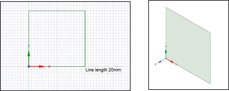
• Select the surface and create a new component ‘air’.
• Create another new component ‘water’ and create a square of 20x20 mm.

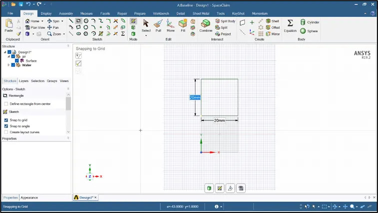
• Now to obtain a conformal mesh, select the geometry and under ‘workbench’ click ‘share’.

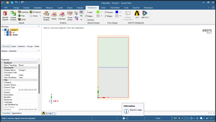
Meshing:

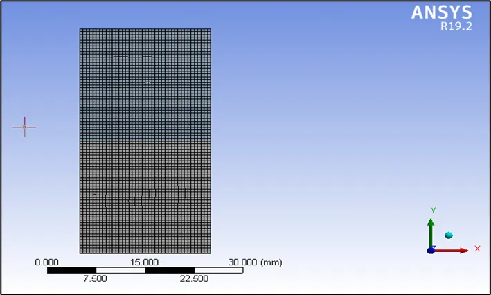
• Set the element size to 0.5 mm and generate the mesh.
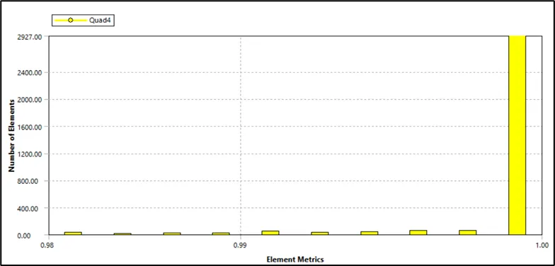
• The generated mesh has 3200 quadrilateral elements with an average quality of 0.99872.

Simulation setup:

General settings

• Solver type: Pressure based
• Time: Transient
• Velocity formulation: Absolute
• Enable ‘gravity’ and enter a value of -9.81m/s² in Y direction.

Physics settings

• Viscous model: Laminar (assuming the velocity is slower)
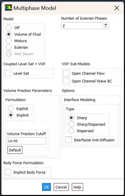
• Click on multiphase model and enable ‘Volume of Fluids’ (VOF).
• The implicit formulation is used with two Eulerian phases i.e., water and air.

Materials

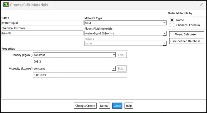
• Under ‘fluid’ material type, add ‘water liquid’ from fluent data base.

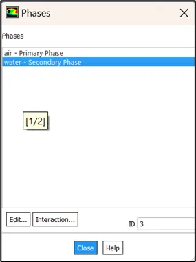
• Click on ‘Show/list all phases and name air as ‘primary phase’ and water as ‘secondary phase’.

• Since there are no named surfaces, confirm the air and water surfaces using ‘mesh display’ option.

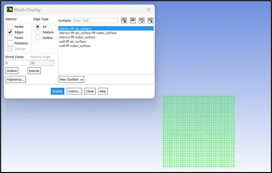
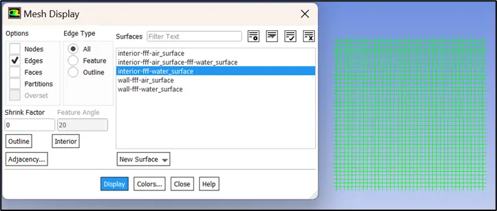
• Next step is patching (assigning properties to selected regions).
• Before patching, initialize the solution using standard initialization.
• Click on ‘patch’ and select ‘water’ under ‘phase’ menu, variable as ‘volume fraction’ with a value of 1, select ‘water surface’ zone and click on patch. Similarly, select air surface and enter value as 0 and patch.

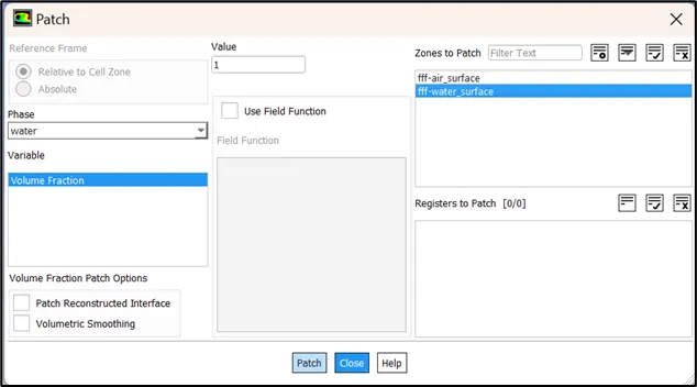
• The ‘value’ here means ‘alpha’ which represents the two phases. For instance, when solution is initialized, alpha = 1 indicates, water only at the top and alpha = 0 indicates no water/only air at the bottom.
• To verify the initialization to be correct, create a contour under post-processing for volume fraction of water.

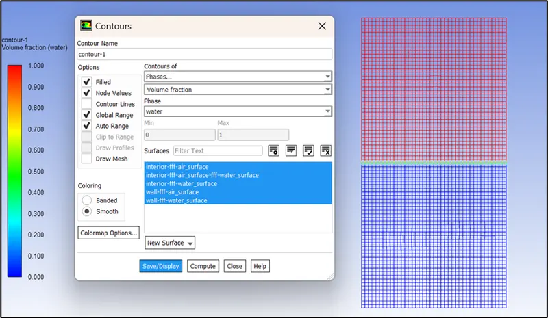
• The volume fraction of 1 at the top suggests that the setup is correct.
• Create an animation to observe the contours.

Solving:

• Set the time step to 0.005 and number of time steps to be 1000, i.e., 5 seconds of total run time and click on calculate.

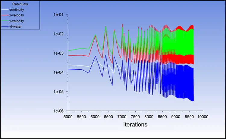
Residual plot

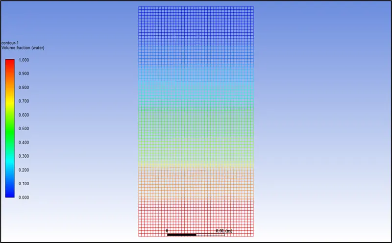
Volume fraction contour plot

Animation file:

https://drive.google.com/file/d/1qlyc3Ve_qtUcjkCsNOc_MBVRq3L8MriF/view?usp=share_link

Refined mesh

The study is carried out for using the mesh element size of 0.1 mm.

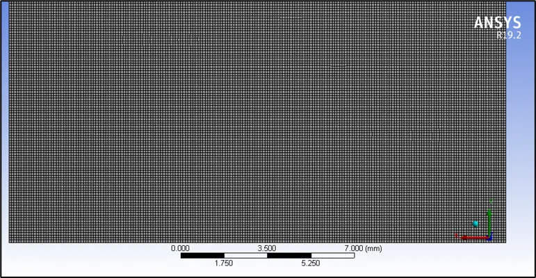
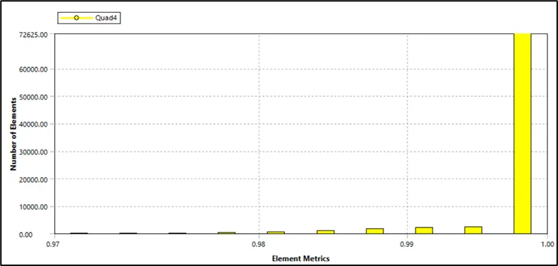
• The mesh contains 80000 elements of quadrilateral type with an average element quality of 0.9985.

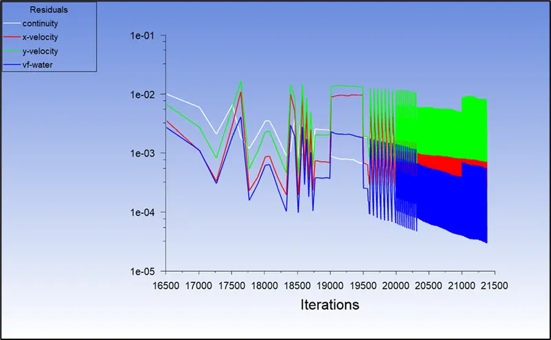
The solution when run with a time step of 0.005 seconds encountered a floating-point error, the solver reached a state where it was not able to compute further. Hence, the time step is reduced to a value of 0.0025.

Residual plot

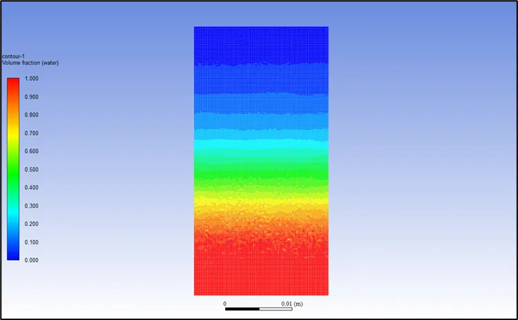
Volume fraction contour plot

Animation file

https://drive.google.com/file/d/1mxPGO8kQEpO5fF1BqPlYWKjlY42E1c2n/view?usp=sharing

User defined material

• Density = 400 kg/m³
• Viscosity = 0.001 kg/m-s

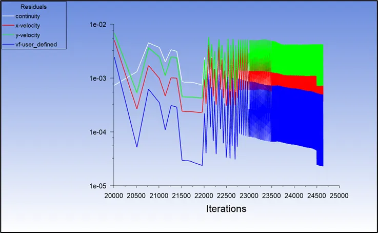
Residual plot

Volume fraction contour plot

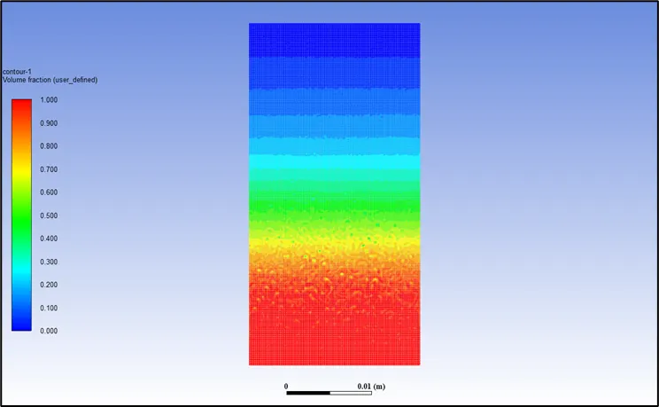
Animation file

https://drive.google.com/file/d/1qMfYJa1JR9QgjmnVaTRHjFFTBN3N7wp4/view?usp=sharing

Results and observations

It can be observed that for the baseline mesh the volume fraction contours are very course and the instability flow cannot be observed clearly. Further, the refined mesh (both air – water and water – user defined) it can be observed that the contours are captured very clearly but the time taken for the simulation is comparatively more i.e., the heavier fluid takes more time to settle down.

Atwood number (A):

It is a dimensionless number used in the study of hydrodynamic instability in density stratified flows (where the density variation is in the vertical direction).

It is a dimensionless density ratio defined as

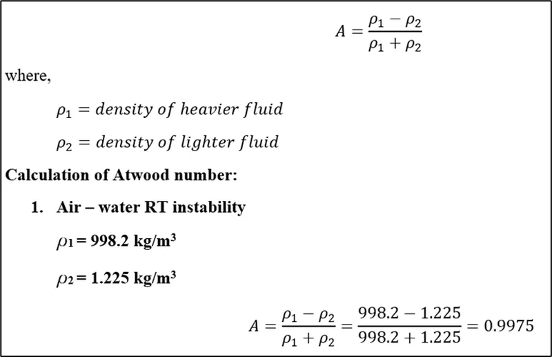
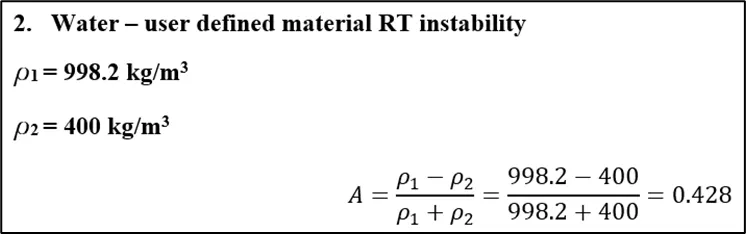
The behavior of the instability is affected by the variation in the Atwood number. In case of air – water RT instability, the value is closer to 1, which can be inferred as the lighter fluid below the heavier fluid takes the form of large bubbles or plumes and in case of user defined – water RT instability, the value is closer to 0, which represents that the instability flows take the form of symmetric fingers.

Reason for performing the study in transient state

Steady state simulations are mainly used when the flow properties are constant and the computation performed by steady state are fully developed solutions meaning they don’t change with time. Also, the solution that we obtain comprises of the mean values that are computed.

In contrast, Transient simulation computes instantaneous values in each time for each quantity. It also helps to capture the flow better and can be used to run the simulation at smaller time steps. In order to observe the instabilities smaller time steps are required which is only possible through transient simulation. Hence, it is more ideal and preferred in the case of RT instability calculations.