Week 5 - Rayleigh Taylor Instability
RAYLEIGH TAYLOR INSTABILITY
AIM: To Perform the Rayleigh Taylor instability simulation for 2 different mesh sizes with the base mesh being 0.5 mm. Compare the results by showing the animations and explaining the results.
Expected results: -
- What are some practical CFD models that have been based on the mathematical analysis of Rayleigh Taylor waves? In your own words, explain how these mathematical models have been adapted for CFD calculations.
- Perform the Rayleigh Taylor instability simulation for 2 different mesh sizes with the base mesh being 0.5 mm. Compare the results by showing the animations (Attach them from your google drive). Observe the differences in the animation and explain the effect of mesh size on simulation. Also, explain why a steady-state approach might not be suitable for these types of simulation. [ Choose Air and Water for this simulation]
- Run one more simulation with water and user-defined material (density = 400 kg/m3, viscosity = 0.001 kg/m-s) for refined mesh.
- Define the Atwood Number. Find out the Atwood number for both the cases and explain how the variation in Atwood number in the above two cases affects the behaviour of the instability.
INTRODUCTION:
The Rayleigh-Taylor instability is a fingering instability of an interface between two fluids of different densities, which occurs when the light fluid is pushing the heavy fluid. Thus, we can infer a simple criterion for the onset of Taylor instability at the interface between two fluids of different densities: If the heavy fluid pushes the light fluid, the interface is stable. If the light fluid pushes the heavy fluid, the interface is unstable.
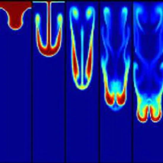
Some of the practical CFD models that have been based on the mathematical analysis of Rayleigh Taylor waves.
Richtmyer–Meshkov instability:
The Richtmyer–Meshkov instability (RMI) occurs when two fluids of different density are impulsively accelerated. Normally this is by the passage of a shock wave. The development of the instability begins with small amplitude perturbations which initially grow linearly with time. This is followed by a nonlinear regime with bubbles appearing in the case of a light fluid penetrating a heavy fluid, and with spikes appearing in the case of a heavy fluid penetrating a light fluid. A chaotic regime eventually is reached, and the two fluids mix. This instability can be considered the impulsive-acceleration limit of the Rayleigh-Taylor instability.
Supersonic combustion in Scramjet may benefit from RMI as the fuel-oxidants interface is enhanced by the breakup of the fuel into finer droplets. Also in studies of deflagration to detonation transistion (DDT) processes show that RMI-induced flame acceleration can result in detonation.
Kelvin-Helmholtz instability:
Fluid Dynamics predicts the onset of instability and transition to turbulent flow within fluids of different densities moving at different speeds. If surface tension is ignored, two fluids in parallel motion with different velocities and densities yield an interface that is unstable to short-wavelength perturbations for all speeds. However, surface tension is able to stabilize the short wavelength instability up to a threshold velocity.
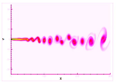
Plateau–Rayleigh instability:
The Plateau–Rayleigh instability, often just called the Rayleigh instability, explains why and how a falling stream of fluid breaks up into smaller packets with the same volume but less surface area. It is related to the Rayleigh-Taylor instability and is part of a greater branch of fluid dynamics concerned with fluid thread breakup. This fluid instability is exploited in the design of a particular type of ink jet technology whereby a jet of liquid is perturbed into a steady stream of droplets.
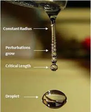
Steps involved in analysis:
- Pre-processing
- Solving
- Post-processing
CASE 1:
To stimulate baseline mesh of 0.5 mm with material properties of air and water.
Pre-processing:
- From the analysis system toolbox open the Fluid Flow (Fluent)
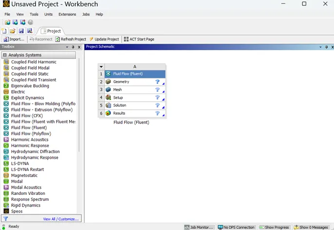
- In Geometry open the spaceclaim for the 2D designing of the model.
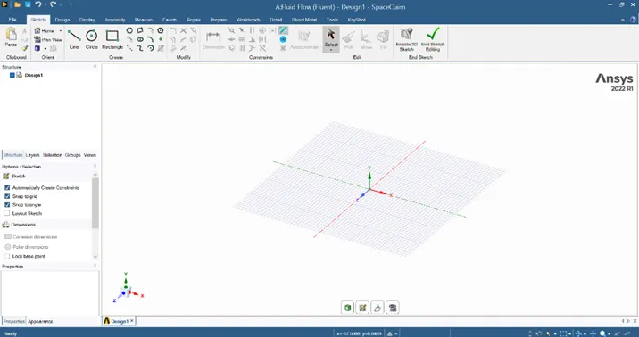
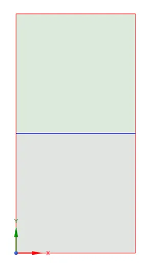
- Create to geometry for air and water.
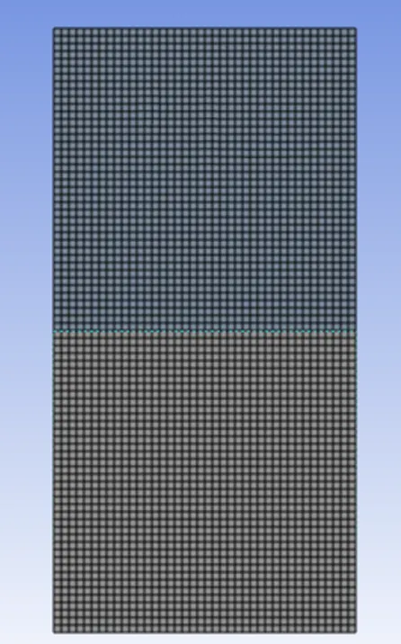
- The baseline mesh is generated for mesh size of 0.5mm.
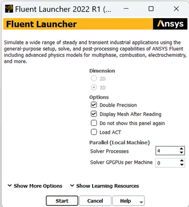
- Solving:
- Open the setup for applying the boundary condition for the fluid flow solution.
|
Setup |
LAMINAR |
|
Solver time |
Transient |
|
Solver type |
Pressure Based |
|
Gravity |
Y = -9.81 |
|
Viscous Model |
LAMINAR |
|
Material |
Air o Density- 1.225kg/m3 o Viscosity - 1.7894e-05 Pa s Water o Density- 998.2kg/m3 o Viscosity – 0.001003 Pa s |
|
Multiphases |
Volume of fluid- Implicit o Primary phase- Air o Secondary phase- Water |
|
Patch |
Air Volume of fraction – 0 Water Volume of fraction – 1 |
|
Run Calculation |
o Timestep size(s) – 0.005 o No. of. timestep - 750 |
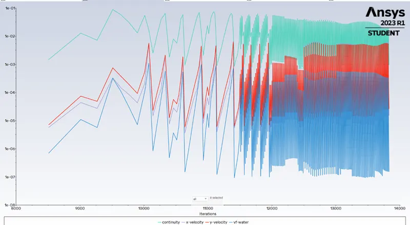
- Scaled residual plots.
- Volume of fraction (Water).
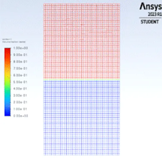
- Link for solution animation of the Volume of fraction (Water).
https://drive.google.com/file/d/1sq7ql9RhQwAWnc_xSTv4Y8oGDiX2mOfn/view?usp=drive_link
CASE 2:
To stimulate refined mesh of 0.3 mm with material properties of air and water.
Pre-processing:
- From the analysis system toolbox open the Fluid Flow (Fluent)
- In Geometry open the spaceclaim for the 2D designing of the model.
- Create to geometry for air and water.
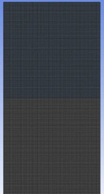
- The baseline mesh is generated for mesh size of 0.3mm.
- Solving:
- Open the setup for applying the boundary condition for the fluid flow solution.
|
Setup |
LAMINAR |
|
Solver time |
Transient |
|
Solver type |
Pressure Based |
|
Gravity |
Y = -9.81 |
|
Viscous Model |
LAMINAR |
|
Material |
Air o Density- 1.225kg/m3 o Viscosity - 1.7894e-05 Pa s Water o Density- 998.2kg/m3 o Viscosity – 0.001003 Pa s |
|
Multiphases |
Volume of fluid- Implicit o Primary phase- Air o Secondary phase- Water |
|
Patch |
Air Volume of fraction – 0 Water Volume of fraction – 1 |
|
Run Calculation |
o Timestep size(s) – 0.005 o No. of. timestep – 750 |
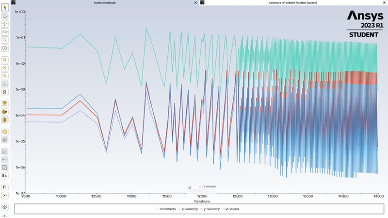
- Scaled residual plots.
- Volume of fraction (Water).
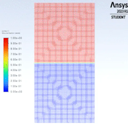
- Link for solution animation of the Volume of fraction (Water).
https://drive.google.com/file/d/1sucO6EA5LLu0_XeIZQhJStDEavfwWZb5/view?usp=drive_link
CASE 3:
To stimulate refined mesh of 0.3 mm with material properties of user-defined and water.
Pre-processing:
- From the analysis system toolbox open the Fluid Flow (Fluent)
- In Geometry open the spaceclaim for the 2D designing of the model.
- Create to geometry for user-defined and water.
- The baseline mesh is generated for mesh size of 0.3mm.
- Solving:
- Open the setup for applying the boundary condition for the fluid flow solution.
|
Setup |
LAMINAR |
|
Solver time |
Transient |
|
Solver type |
Pressure Based |
|
Gravity |
Y = -9.81 |
|
Viscous Model |
LAMINAR |
|
Material |
User-defined o Density- 400kg/m3 o Viscosity – 0.001 Pa s Water o Density- 998.2kg/m3 o Viscosity – 0.001003 Pa s |
|
Multiphases |
Volume of fluid- Implicit o Primary phase- User-defined o Secondary phase- Water |
|
Patch |
User-defined Volume of fraction – 0 Water Volume of fraction – 1 |
|
Run Calculation |
o Timestep size(s) – 0.005 o No. of. timestep – 750 |
- Scaled residual plots.
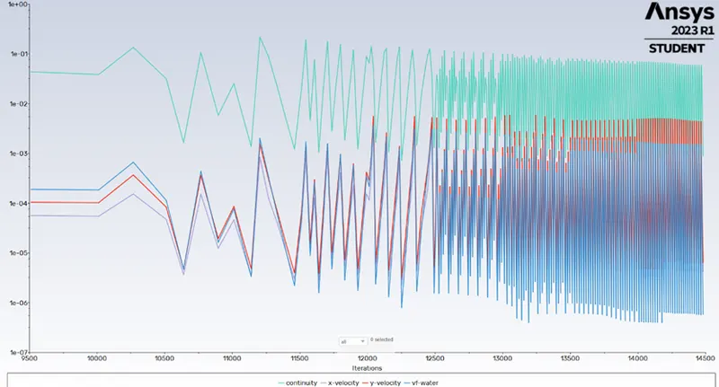
- Volume of fraction (Water).
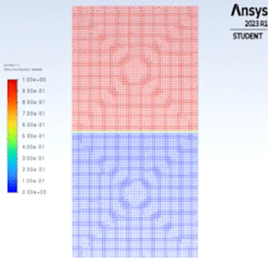
- Link for solution animation of the Volume of fraction (Water).
https://drive.google.com/file/d/1sudzPX5gR8afBGQJoeWCeDf4DRp5sRxr/view?usp=drive_link
Atwood Number:
The Atwood number (A) is a dimensionaless number in fluid dynamics used in the study of hydrodynamic instabilities in density stratified flows. It is a dimensionless density ratio defined as
Where,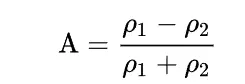
rho1 = density of the heavy fluid
rho2 = density of the light fluid
After calculations Atwood number’s for
Air and water = 0.997
User- defined and water = 0.427
Conclusion:
- From the grid independence study results, I conclude that refining mesh size increases the accuracy of the stimulation results.
- For the refined mesh condition solver takes more time to run the iteration and instabilities occurs slowly in this case. (Mainly in user-defined material)
- When the density of the light fluid is increasing the Atwood number is get reducing. From the calculation air and water density ratio is twice the user-defined and water.so, the Atwood number is more for air and water.
Reference Paper