Week 5 - Rayleigh Taylor Instability

The Rayleigh–Taylor instability, or RT instability:

The Rayleigh–Taylor instability, or RT instability is an instability of an interface between two fluids of different densities which occurs when the lighter fluid is pushing the heavier fluid. Water suspended atop oil is an everyday example of Rayleigh–Taylor instability, and it may be modeled by two completely plane-parallel layers of immiscible fluid, the denser fluid on top of the less dense one and both subject to the Earth's gravity. The equilibrium here is unstable to any perturbations or disturbances of the interface: if a parcel of heavier fluid is displaced downward with an equal volume of lighter fluid displaced upwards, the potential energy of the configuration is lower than the initial state.

multi-phase models

Homogenious models:

A:Volume flow models:The VOF model can model two or more immiscible fluids by solving a single set of momentum equations and tracking the volume fraction of each of the fluids throughout the domain. Typical applications include the prediction of jet breakup, the motion of large bubbles in a liquid, the motion of liquid after a dam break, and the steady or transient tracking of any liquid-gas interface.

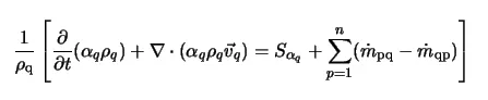
where `underset(pq)(dotm)` is the mass transfer from `q` phase to phase `p` and `underset(qp)(dotm)` is the mass transfer from `p` phase to phase `q` . By default, the source term on the right-hand side of Equation , `underset(alpha q)(s)` , is zero, but you can specify a constant or user-defined mass source for each phase. for more information on the modeling of mass transfer in ANSYS Fluent general multi phase models.

the Mixture Model:The mixture model is a simplified multi-phase model that can be used in different ways. It can be used to model multi-phase flows where the phases move at different velocities, but assume local equilibrium over short spatial length scales. It can be used to model homogeneous multi-phase flows with very strong coupling and phases moving at the same velocity and lastly, the mixture models are used to calculate non-Newtonian viscosity.

The mixture model can model phases (fluid or particulate) by solving the momentum, continuity, and energy equations for the mixture, the volume fraction equations for the secondary phases, and algebraic expressions for the relative velocities.

The continuity equation for the mixture is:

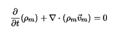
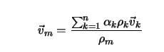
where `underset(m)(vecv)` is the mass-averaged velocity:

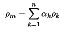
is the mixture density:

the Wet Steam Model:During the rapid expansion of steam, a condensation process will take place shortly after the state path crosses the vapor-saturation line. The expansion process causes the super-heated dry steam to first sub-cool and then nucleate to form a two-phase mixture of saturated vapor and fine liquid droplets known as wet steam.

The wet steam is a mixture of two-phases. The primary phase is the gaseous-phase consisting of water-vapor (denoted by the subscript v) while the secondary phase is the liquid-phase consisting of condensed-water droplets (denoted by the subscript l).

The following assumptions are made in this model:

• The velocity slip between the droplets and gaseous-phase is negligible.
• The interactions between droplets are neglected.
• The mass fraction of the condensed phase, (also known as wetness factor), is small ( `beta<20`).
• Since droplet sizes are typically very small (from approximately 0.1 microns to approximately 100 microns), it is assumed that the volume of the condensed liquid phase is negligible.

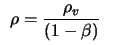
From the preceding assumptions, it follows that the mixture density ( ) can be related to the vapor density ( ) by the following equation:

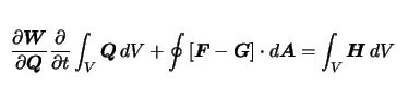
Navier-Stokes equations:

Non Homogenious models:

the Eulerian Model:With the Eulerian multi-phase model, the number of secondary phases is limited only by memory requirements and convergence behavior. Any number of secondary phases can be modeled, provided that sufficient memory is available. For complex multi-phase flows, however, you may find that your solution is limited by convergence behavior. See this section in the separate User's Guide for multi-phase modeling strategies.

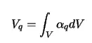
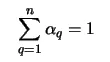
The description of multi-phase flow as interpenetrating continua incorporates the concept of phasic volume fractions , denoted here by . Volume fractions represent the space occupied by each phase, and the laws of conservation of mass and momentum are satisfied by each phase individually. The derivation of the conservation equations can be done by ensemble averaging the local instantaneous balance for each of the phases or by using the mixture theory approach.

The volume of phase , , is defined by:

Geometery:

1. Create a square in XY-plean of 20m
2. By using the pull tool make them surface.
3. Create a new component then create a square top of the previous square.Then make the rectangle in plane.

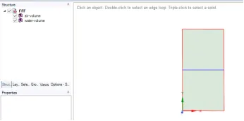
1. Then name them as air volume and water volume.
2. Using the shear property,shear the property of the interference line, it helps to creat a conformal mash.

Mesh:

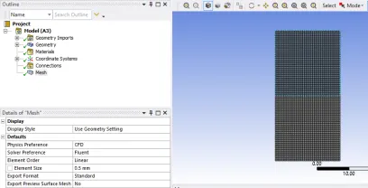
Do the mashing with 0.5mm (here total no of mash is 3200) element size, then check the mash is conformal or not.

Setup:

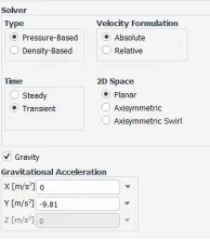
Here we use pressure based transient solver is used

Steady flow: in this we take all the properties like temperature ,density, pressure are constant with time in a control surfaces.

Transient flow: in this we take all the properties like temperature ,density, pressure are change with time in a control surfaces.so for that we have to calculate all the value for every instant of time. Here fluid mixing take place ,so the properties are changing with every instant of time, In transient solver we solve all the properties of every instant of time at all the nudes.

Here we click the gravity because gravity is the only force here.And the gravity is act in -ve y direction.

Models: Here we use use only multi phase model because here fluid is in two different phase.

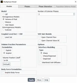
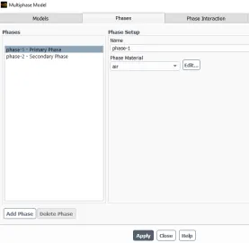
1. Here we use volume of fluid model with implicitly and set the Eulerian phase in 2, because here we use two different immiscible fluid ,so we do the volume fraction model. And air and water used here ,so two phase is use .
2. In Phase we describe the phase material as per the phase ,In phase 1 we set the material as air in phase 2 we set the material as water_liquid.Before set the phase we should set the materials.

set the materials:

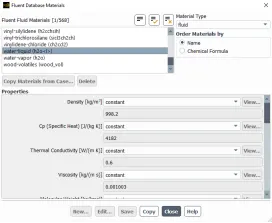
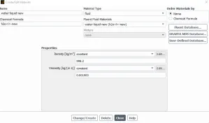
1. Set the material properties as water fluid .
2. Syntex: fluent database >>search (water-fluid)>>select water liquid(deselect others )>>copy>>close>>create and close >>close.

Initialization:

Here we have to describe the water and air amount as per the volume initially,so we do the standard initialization and set the patch.

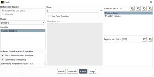
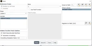
1. Zone paach>>air-volume, phase>>phase-1,select volume fraction and set the volume fraction at the Zero
2. It Describe that in air volume aria phase-2(water) amount is 0%. simlerly set the value of the water-volume as 1.

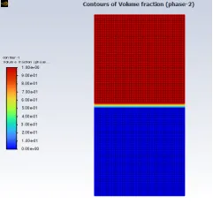
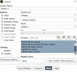
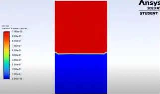
Then create a couture of volume fraction(phase) to check the patch is OK or not. It show the upper part is full of water and lower part is full of air.

Then create animation to track the diffusion processes.

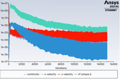
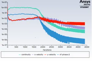
Here the the solution continuously divergent as the iteration get progressed.

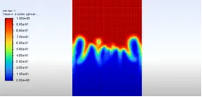
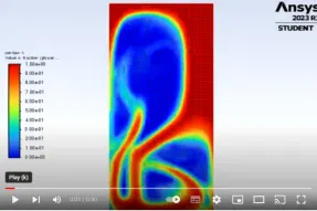
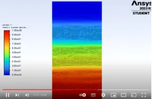
animated vedio.

https://youtu.be/7DgCU7YSCz4

For mash 1mm:

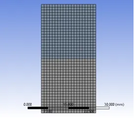
Create element size 1mm mash now total no elements is 800

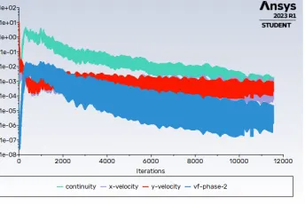
Divergence Decreases in increase with the in mash.

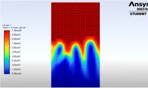
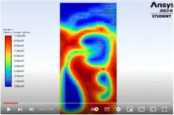
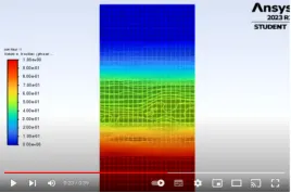
• Mixing was not perfect and take very less time to mix up.

Animation vedio

https://youtu.be/6gpJGgJ9Zbs

Mash 0.25mm

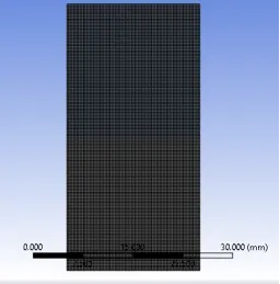
Create mash of 0.25mm and Total Element 12800

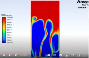
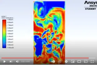
• The perfect mixing is taking place and take higher time to get the stability.

Animation vedio.

https://youtu.be/kzetkSQKxzw

Mash 25mm with user specified material:

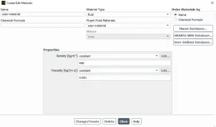
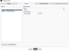
Now Create a user specified material and set the density at 400kg/m^3 and viscosity is 0.001kg/m-s.

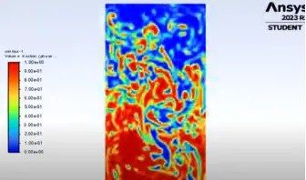
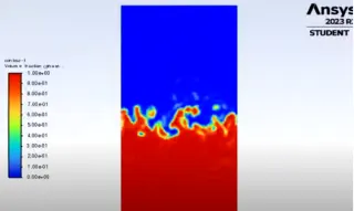
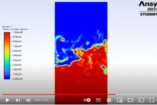
• Here it take very less time to stable but after some time it become unstable.
• Here initially created bobbles are small as compere to the bobbles create in air

Animation 4

https://youtu.be/CIl_r3GKE0M

Atwood No:

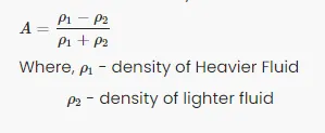
It is a dimensionless no, which is defined by A

Mash size	Total no mash element	Density of lighter element	Atwood no
1mm	800	1.225Kg/m^3	0.9975
0.5mm	3200	1.225Kg/m^3	0.9975
0.25mm	12800	1.225Kg/m^3	0.9975
0.25mm	12800	400kg/m^3	0.427

The density of water was 998.2Kg/m^3

• Here we analyze that The Atwood no was nearly one for air as lighter fluid and nearer to zero for user define material.
• For air as lighter material the density deference is very high,so air is creating big baubles initially and take higher time to mix-up.
• For user define material it create small bobbles and take very less time to mix up ,because the he density deference is very lower then air And it take very less time to mix up.

Conclusion:

1. Here we use the transient,Because the properties are changing with time in the control volume .Here inside the control volume a mixing processes was taken place so we have to track the amount of air and water inside the small control volume (Inside the mash) ,we have to count with time.Then also we track the fluid motion and how much time take to be stable.
2. Here we done the simulation in three diffrent mashing 1mm,0.5mm,0.25mm, in all the three process the motion and mixing process are same for all but for lower mash size it takes more time to stable.So in lower mash the instability was captured properly.
3. In higher density material (user define material) it create small baubles,and mixing was very fast.
4. Atwood number is very lower for the higher density material ,because density difference was very high.So It is more difficult to compress the user define material by water then air, so In user define material create small baubles.