Week 5 - Rayleigh Taylor Instability
imeAIM
To perform Rayleigh Taylor instability simulation and explain the results.
Rayleigh Taylor Instability
The Rayleigh–Taylor instability, or RT instability, is an instability of an interface between two fluids of different densities which occurs when the lighter fluid is pushing the heavier fluid. Examples include the behavior of water suspended above oil in the gravity of Earth, mushroom clouds like those from volcanic eruptions and atmospheric nuclear explosions, supernova explotions which expanding core gas is accelerated into denser shell gas,instabilities in plasma fusion reactors and inertial confinement fusion.
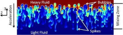
When two fluids of different density are suspended over one other, with the heavier fluid being on top of the lighter fluid, an instability is caused at the interface due to the bouyant and gravity forces acting.
Practical CFD models that have been based on mathematical analysis of RT waves
- Kelvin-Helmholtz instability
- Richtmyer-Meshkov instability
- Plateau-Rayleigh instability
Kelvin-Helmholtz instability
The Kelvin–Helmholtz instability is a fluid instability that occurs when there is velocity shear in a single continuous fluid or a velocity difference across the interface between two fluid. Kelvin-Helmholtz instabilities are visible in the atmospheres of planets and moons, such as in cloud formations on Earth or the Red Spot on Jupiter, and the atmospheres of the Sun and other stars.
Richtmyer-Meshkov instability
The Richtmyer–Meshkov instability (RMI) occurs when two fluids of different density are impulsively accelerated. Normally this is by the passage of a shock wave. The development of the instability begins with small amplitude perturbations which initially grow linearly with time. This is followed by a nonlinear regime with bubbles appearing in the case of a light fluid penetrating a heavy fluid, and with spikes appearing in the case of a heavy fluid penetrating a light fluid. A chaotic regime eventually is reached and the two fluids mix. This instability can be considered the impulsive-acceleration limit of the Rayleigh–Taylor instability.
Plateau-Rayleigh instability
The Plateau–Rayleigh instability, often just called the Rayleigh instability, explains why and how a falling stream of fluid breaks up into smaller packets with the same volume but less surface area. It is related to the Rayleigh–Taylor instability and is part of a greater branch of fluid dynamics concerned with fluid thread breakup. This fluid instability is exploited in the design of a particular type of ink jet technology whereby a jet of liquid is perturbed into a steady stream of droplets. The driving force of the Plateau–Rayleigh instability is that liquids, by virtue of their surface tensions, tend to minimize their surface area
Atwood Number
- The Atwood number is a dimensionless number in fluid dynamics used in the study of hydrodynamic instabilities in density-stratified flows. The Atwood number equals the ratio of the difference in mass densities to their sum.
`A= (rho1-rho2)/(rho1+rho2)`
Atwood number is an important parameter in the study of Rayleigh–Taylor instability and Richtmyer–Meshkov instability. In Rayleigh–Taylor instability, the penetration distance of heavy fluid bubbles into the light fluid is a function of acceleration time scale, Ag`t^2` where g is the gravitational acceleration and t is the time.
Steady state simulation cannot be done on Rayleigh Taylor instability since the instability happens with respect to time and hence time function is important to capture the essential features of the simulation.
Procedure
- Open Fluent workbench
- Open spaceclaim.
- Draw a rectangle of 20 mm x 20 mm.
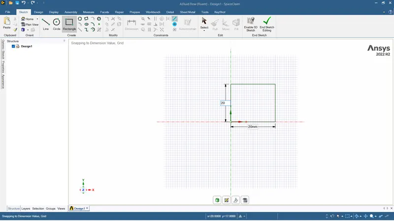
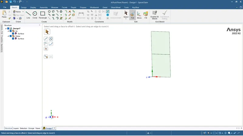
- Use pull tool to create a surface.
- Move the surface into a new component.
- Create another surfcace under a new component.
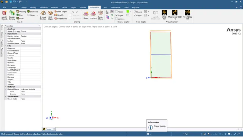
- Use workbench>share option so that information transfer happens between shared interfaces.
- close spaceclaim and open fluent mesh.
- Create a baseline mesh of element size 0.5 mm.
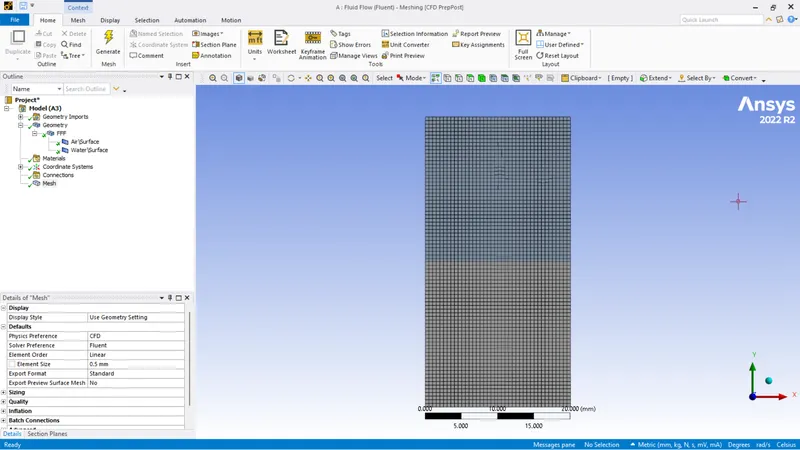
- Open setup with double precision.
Solver Pressure based Velocity formulation Absolute Time Transient Gravity -9.81 m/s in the y axis viscous model Laminar Multiphase Volume of fluid; Implicit; 2 Eulerian phases Materials Air and Water Cell zones Water in water surface and air in air surface Solution SIMPLE Initialization Standard - The phases were updated with air as primary phase and water as secondary phase
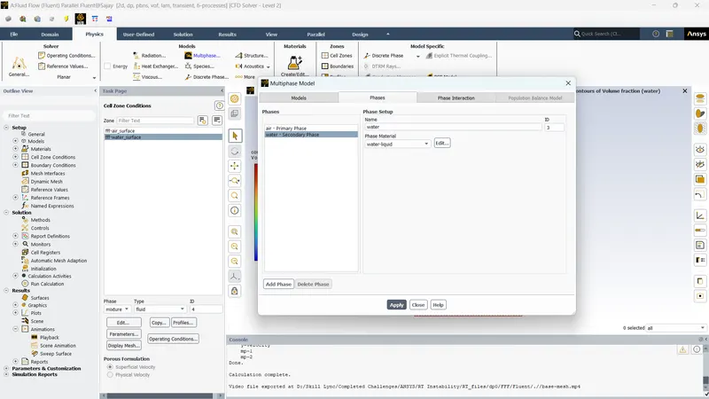
The solution was initialized using standard initialization.
Patching was done with volume fraction and phase as water with value 1 at water surface and 0 at air surface.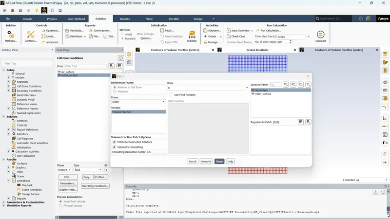
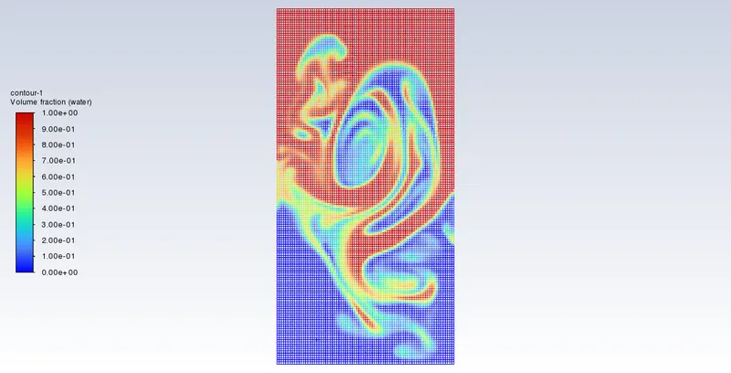
The solution was run with 0.005s time step size for 1000 time steps.
Animation file for base mesh : https://drive.google.com/file/d/1ZJ9KDmvlRmLQu9dSBDdYzQ-hWzNg--bn/view?usp=sharing
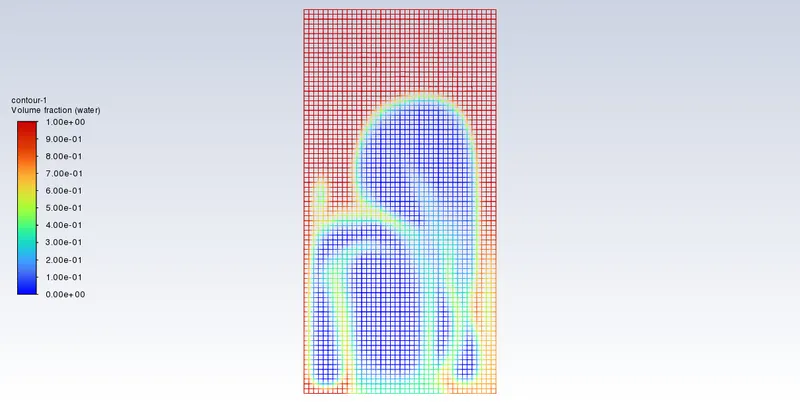
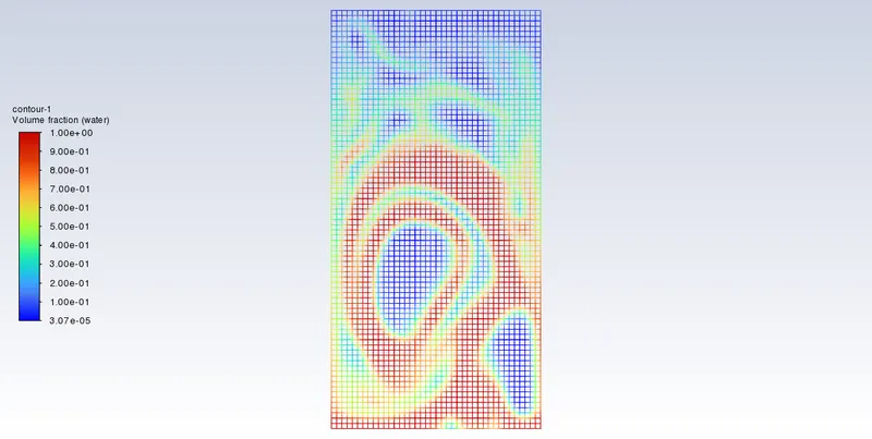
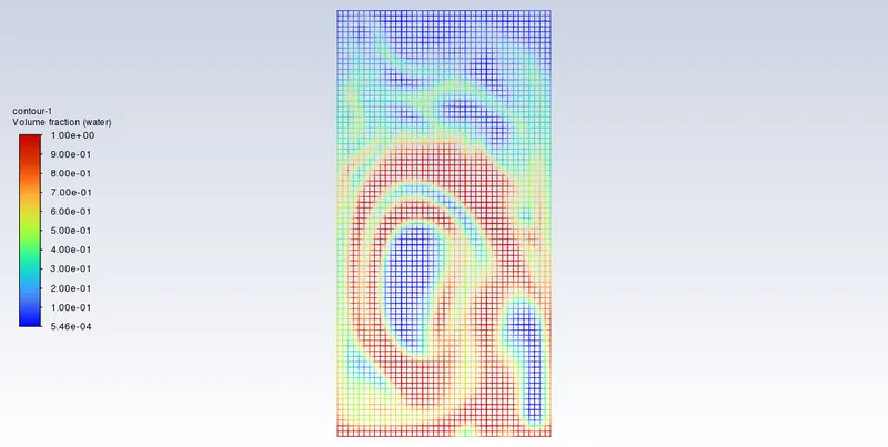
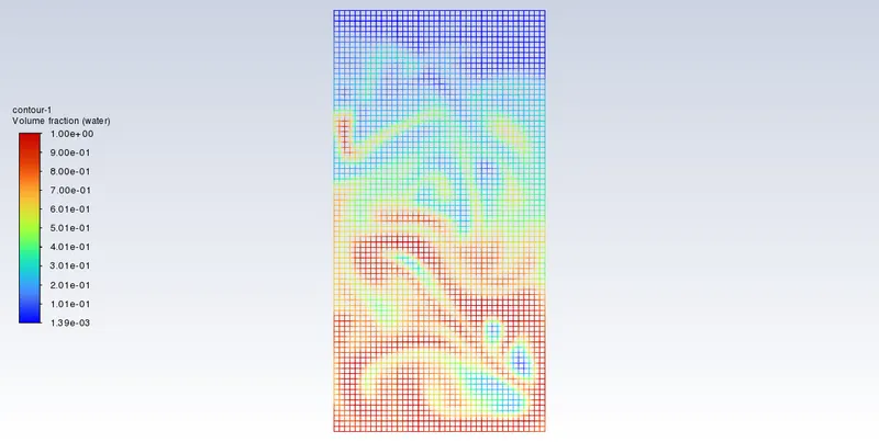
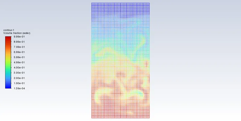
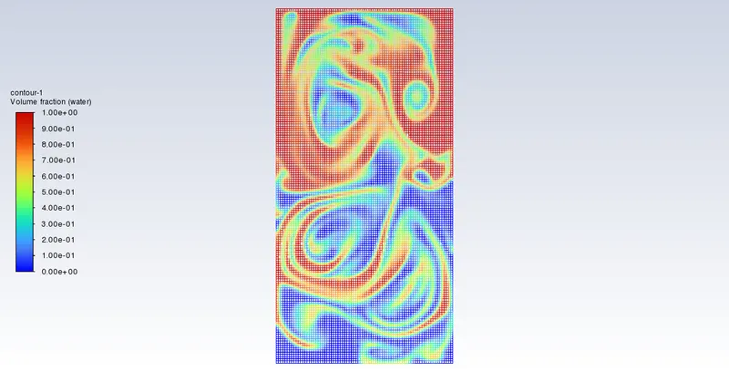
The same setup was run with a mesh size of 0.25 mm
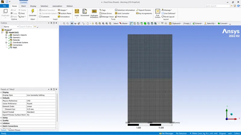
The solution was initialized using standard initialization and patching was done.
The solution was run for 1000 time steps with 0.005s time step size
Animation of fine mesh : https://drive.google.com/file/d/1HsA5rKv_W3eWWXfAYzwANcL0knbvd1g3/view?usp=sharing
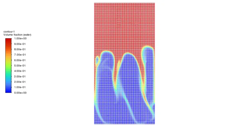
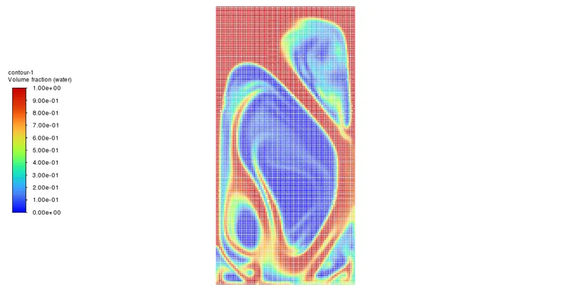
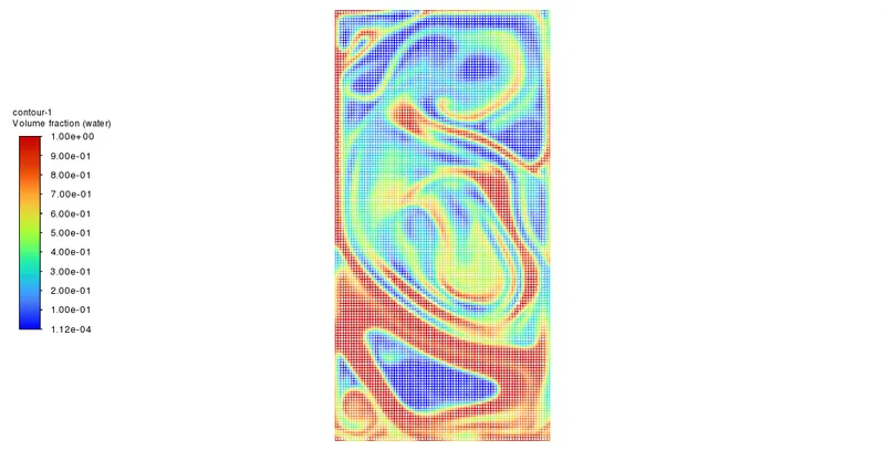
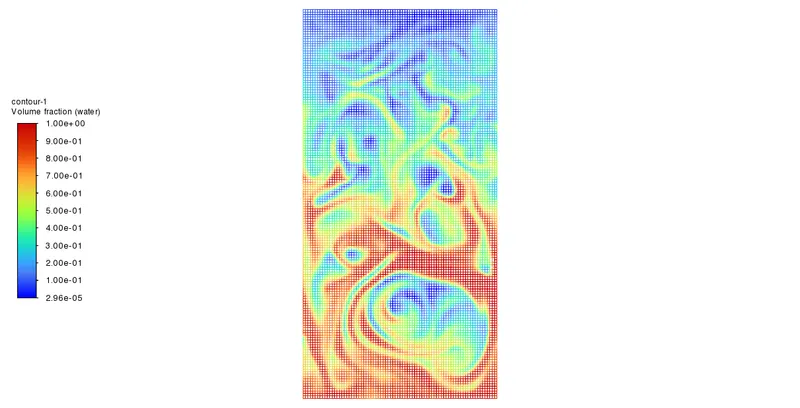
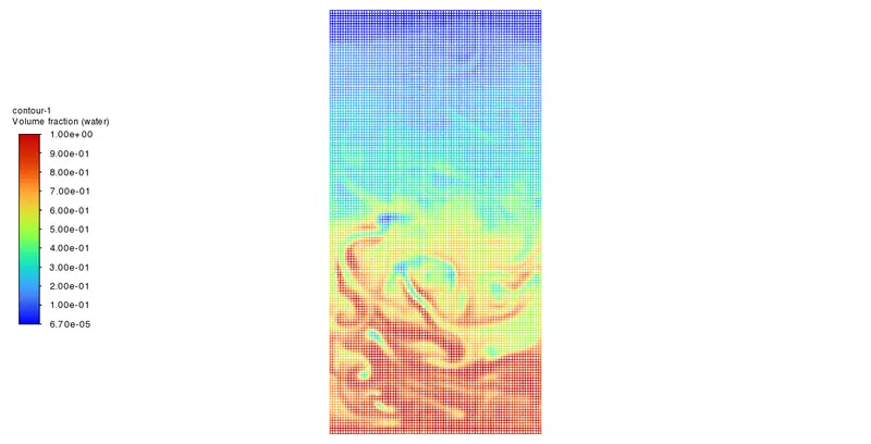
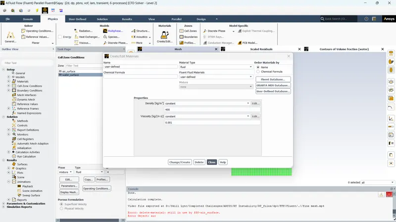
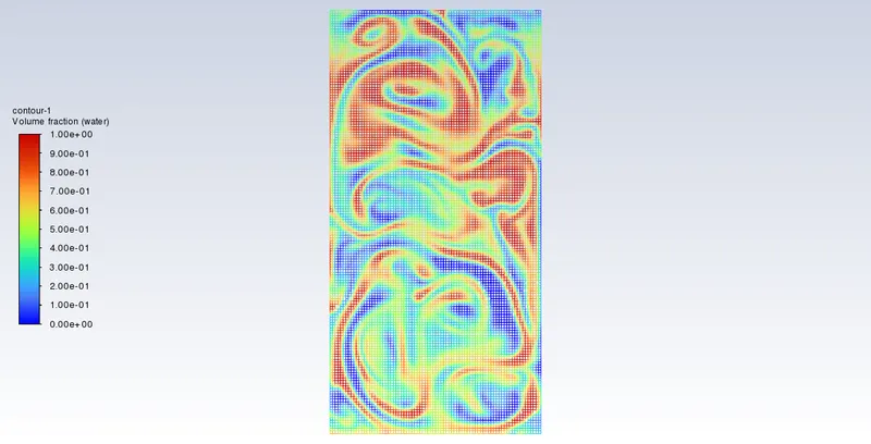
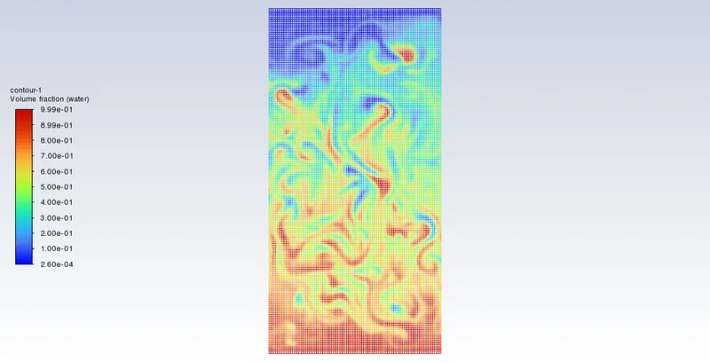
Air was replaced by user defined material having density of 400 kg/m3 and viscocity of 0.001 kg/ms in the fine mesh setup and the solution was run for 1000 time steps with 0.005 s time step interval using standard initialization.
Animation file for user defined medium : https://drive.google.com/file/d/1r-H0JX9Ef1ICFBEPO8u1aja1k-CjGXdS/view?usp=sharing
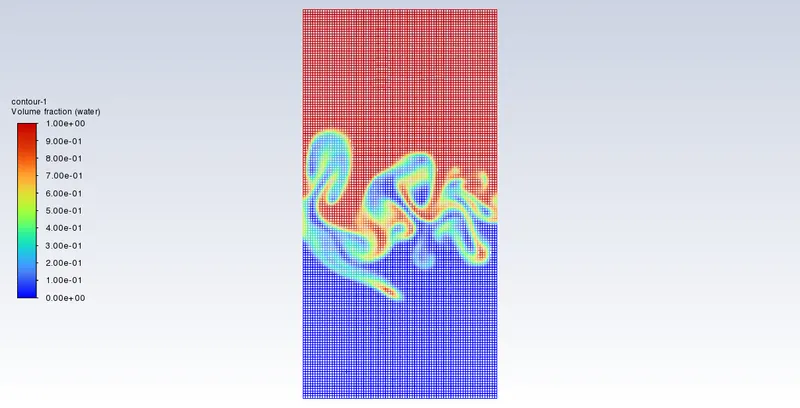
Conclusion
- Atwood number for air and water as the medium, A= 0.997
- Atwood number for water and user defined fluid as medium, A =0.428
- Transient simulation shows that as the atwood number lowered, the instabilities lasted longer. Vortices were present in user defined fluid and water interaction for much longer period than the interaction with water and air.
- Atwood number can be used to define the intensity of the instabilities
- Air water interaction lasted for a short time and the instabilities settled quickly.
- Refining the mesh improved the definitions of the instabilites and gave a much better visualization.
- The computational time was also increased while refining the mesh.