Week 5 - Rayleigh Taylor Instability

AIM:  

Rayleigh- Taylor instability is caused because of heavier fluid above a lighter fluid which makes the interface unstable and the heavier fluid spikes into the lighter fluid and lighter fluid moves above so as to minimise the net potential energy of the system.

• Kelvin–Helmholtz instability: When there is velocity shear on a liquid, velocity difference between interface of two liquids. It is commonly found in earth’s atmosphere and oceans also.
• Richtmyer–Meshkov instability: The Richtmyer–Meshkov instability (RMI) occurs when two fluids of different density are impulsively accelerated. Normally this is by the passage of a shock wave. The development of the instability begins with small amplitude perturbations which initially grow linearly with time. This instability can be considered the impulsive-acceleration limit of the  raylrigh taylore instability
• Plateau–Rayleigh instability: This explains how a liquid stream falling divides itself in smaller fluid particles.  This occurs due to surface tension, which acts to break a cylindrical jet into a stream of droplets having the same total volume but higher surface area. Example-Water coming from a faucet, inkjet printing.

Steady state approach is not desirable here because we are interested in changes that occur in the process and not the final result.

Simulation:

Geometry

Create a rectangle -20mmx20mm. Move this to a component and create similarly another rectangle. One is air one is water.

Workbench> select both boxes>share (share topology automatically becomes share).

Mesh

Mesh size 0.5mm for case 1 and 0.2mm (check if no. of elements exceeds half-million).

Case1 -Mesh size 0.5mm with water and air.

Case 2-Mesh size 0.2mm with water and air.

Case3-Mesh size 0.2mm with water and a user defined material  for density = 400 kg/m³, viscosity = 0.001 kg/m-s).

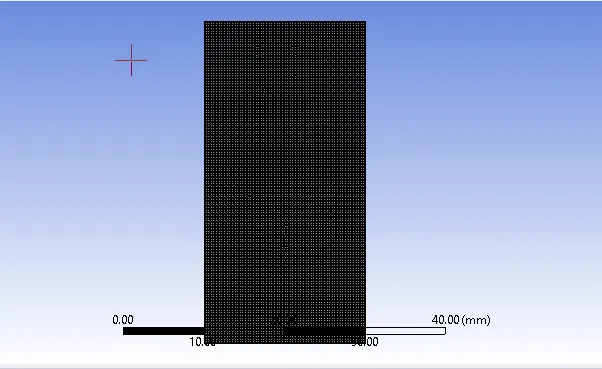
mesh =0.2mm

set-up

1. Select transient method, pressure-based solver and gravity acting in -9.81m/s² in y direction (+ y direction is considered upwards in fluent).
2. Select the laminar flow model. Now select ‘volume of fluid’ method in multi-phase having 2 eulerian phases (here air and water). We use the implicit method.
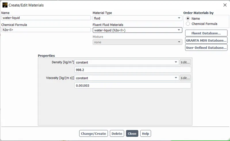
3. Create material – air is already present as a material and hence we choose second phase material (water or user defined other material) and copy it from the fluent data base.
4. Now we are ready to list phases as air and water. This is a very important step. Rename the phases and choose the material for that phase from the drop-down option.
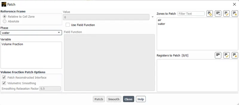
5. Now initialize the solution and patch.
6. Here in patch, volume fraction of water phase in water is 1 and volume fraction of water in air phase is 0.
7. Create a contour for phase to check this.
8. Create a solution animation for contour of water phase also.
9. Autosave animation frst and then see in computational fluid dynamics post once simulation calculation is over.
10. Run the calculation for 1500-time steps with a step size of 5e-3.

                                         

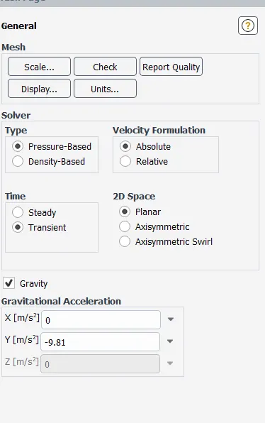
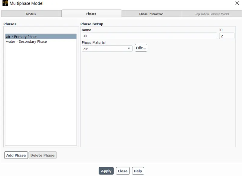
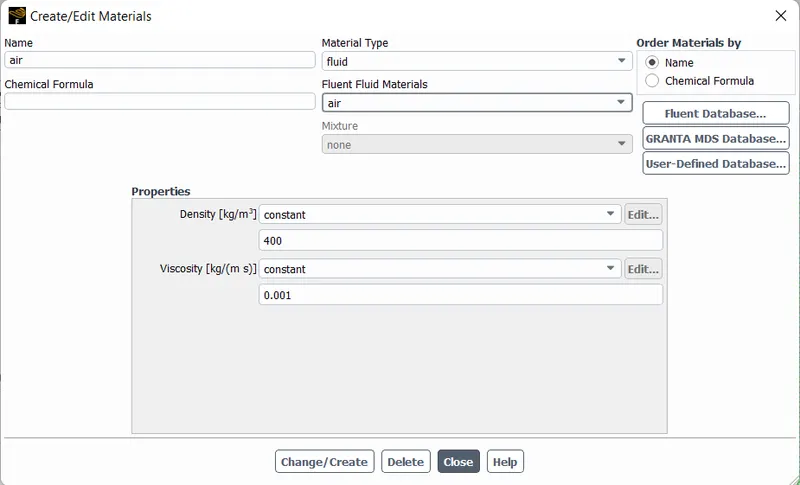
                                                                          Fig: 1st Mateials

                              

 Water and air case setup :

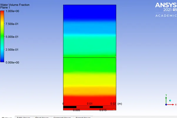
Case1-Results for Mesh size 0.5mm for air and water setup:

 

Eventually the water having higher viscosity than air settles down and air comes up(where volume fraction of water is 0).

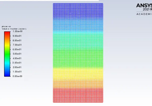
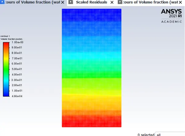
Case 2- Air and water mixture-mesh size 0.2mm

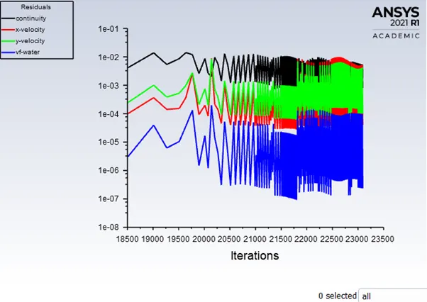
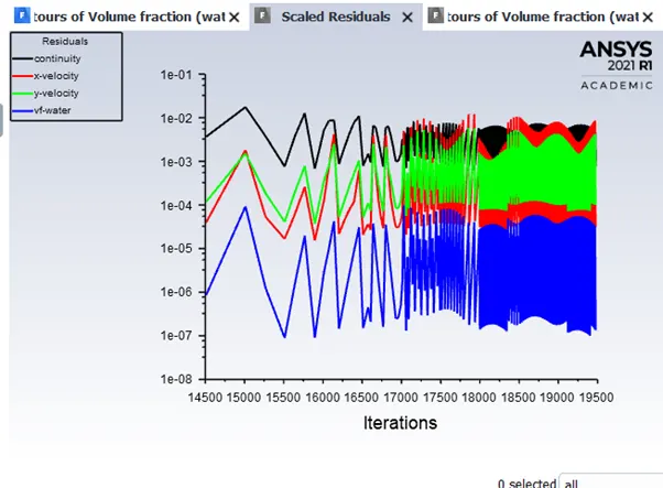
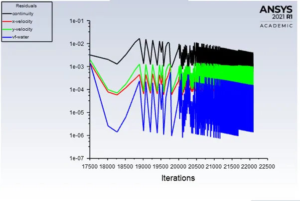
Residual:

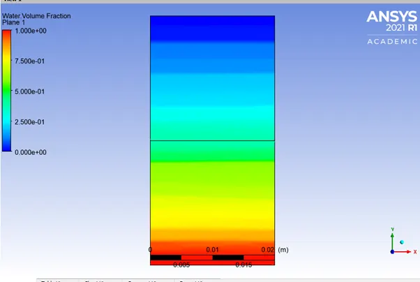
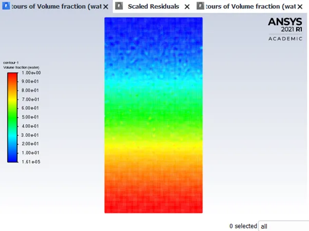
Case3:User defined material and water case setup-

Density-400kg/m3

Volume fraction for water in a mixture of user defined material and water :

Residual:

4. Atwood number(A)= Difference of density of two phases involved/Sum of density of two phases involved.

Air density=ρa=1.225

Water density=ρw=998.2

User defined density=ρu=400

Atwood number for air and water

A=(ρw-ρa)/(ρw+ρa)=998.2-1.225/998.2+1.225=996.975/999.425=0.9975

Atwood number for water and user material

A==(ρw-ρu)/(ρw+ρu)=998.2-400/998.2+400=598.2/1398.2=0.42

For A close to 0, RT instability flows take the form of symmetric "fingers" of fluid; for A close to 1, the much lighter fluid "below" the heavier fluid takes the form of larger bubble-like plumes. This should happen in case of air and water.

 Observation:

• Finer mesh captures the instability better than the coarse mesh, but it takes more time for the heavier fluid to settle down. So it is computationally expensive but produces results with better accuracy.
• The simulation involves capturing instabilities which are changing in an unpredictable manner as a function of time, transient approach is preferred over steady state approach.

Conclusion:

• Atwood number forms a basis to compare and study research paper based on RT instability. Thus we can use these papers to validate our results for better accuracy.