Week 5 - Rayleigh Taylor Instability

Aim :

To Perform the Rayleigh Taylor instability simulation for 2 different mesh sizes with the base mesh being 0.5 mm.

Objectives :

1. What are some practical CFD models that have been based on the mathematical analysis of Rayleigh Taylor waves? In your own words, explain how these mathematical models have been adapted for CFD calculations.
2. Perform the Rayleigh Taylor instability simulation for 2 different mesh sizes with the base mesh being 0.5 mm. Compare the results by showing the animations( Attach them from your google drive). Observe the differences in the animation and explain the effect of mesh size on simulation. Also, explain why a steady-state approach might not be suitable for these types of simulation.[ Choose Air and Water for this simulation]
3. Run one more simulation with water and user-defined material (density = 400 kg/m³, viscosity = 0.001 kg/m-s) for refined mesh.
4. Define the Atwood Number. Find out the Atwood number for both the cases and explain how the variation in Atwood number in the above two cases affects the behavior of the instability.

Introduction :

Rayleigh-Taylor Instability :

• In Multiphase flow, the dynamic variables like the velocity, viscosity, pressure and density are generally used to explain the movement of fluids under the gravitational field.
• Multiphase flows takes place in nuclear geothermal power plants, food processing industries and many others. One of the basic example is Rayleigh Taylor Instability.
• The Rayleigh Taylor Instability is a hydrodynamic instability arises when a high density fluid is placed over a low density fluid in a gravitational field and the two fluids must be immiscible.
• Intially at time t= 0, the system of two fluids is in hydrostatic equlibrium. The pressure gradients are balanced and fluid is in static equilibrium.
• When the density interface is disturbed, the hydrostatic pressure is generated, so the heavier fluid moves downwards and mixes with the lighter one, with the amplitude of perturbation initially growing exponentially but after sometime saturates and forms characteristic mushroom shape.
• When a heavier fluid is displaced downward with an equal volume of lighter fluid displaced upwards, it results in decrease of potential energy than it’s initial state.
• This RTI has been applied to a wide range of problems including the mushroom clouds like volcanic eruptions, nuclear explosions and plasma fusion reactors instability.

Atwood Number :

Dealing with mixtures of fluid one uses the Atwood number to characterize the density difference between two fluids.

Assume that ρ2 is the density of the heavier fluid.
The definition is: At = ρ2−ρ1/ρ2+ρ1.

• For big density differences At tends to 1.
• For small differences At tends to zero.

Literature Studies made :

• The RTI phenomenon was initially introduced by Rayleigh 1883 and later was observed for all accelerated fluids by Taylor 1950.
• Budiana et al. 2020 in their study observed that the evolution of the interface grows faster with the increase in Atwood Number for which in this study the Atwood Number is keptas high as possible in Case 1A. It was seen that with larger Atwood Number, larger amplitude of perturbations are observed. It is due to the larger density ratio of the two fluids, the stronger is the force to develop the interface instability.
• volume of fluid methods(Hirt and Nichols 1981, Gopala and BGMvan 2008, Raessi et al. 2010) and phase field methods(Dinget al. 2007, Chiu and Lin 2011, Lee et al. 2011, Kim 2005).
• Gou et al. 2018 used the multiphase moving particle semi-implicit(MMPS) with periodic boundary conditions to simulate RTI of the immiscible two phase incompressible fluid. The effect of initial perturbation wavelength, surface tension and Atwood Number was investigated in the single mode RTI problem and it was observed that the numerical results were in good agreement with the analytical results.
• Indrashis Saha 2020 study of Rayleigh Taylor Instability with the help of CFD simulation and was well validated with experimental results.

Why not steady-state calculation?

The steady state calculations are useful when the study is focused on to calculate / simulate the end results. Here in this study, the instabilities information is sensitive and completely time-dependent. At each and every time step, the instabilities grow exponentially. Though steady state simulation is capable to capture those instabilities but the results would not be time-accurate. Anyways transient state calculation with reduced time-steps can capture these instabilities at each and every time-steps and sensible time dependent results can be obtained.

Create Geometry:

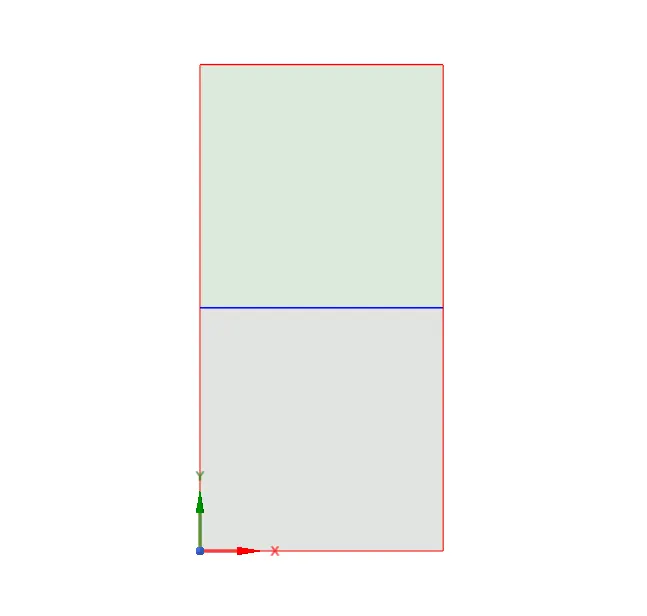
• Create new component and name it air.
• Draw a square of lenght 20 mm x 20 mm and then select pull tool.
• Now again create new component and name it water. Draw a similar square with same dimensions on the top of air component.
• Do share topology.
• Top square is water and bottom square is air.

Mesh :

The Atwood Number for Air-water RT instability

A=(998.2 - 1.225) / (998.2+1.225)

we get A=0.9975

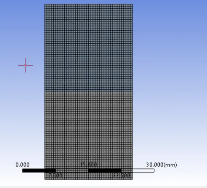
Case 1 :

MESH	Coarse
ELEMENT SIZE	0.5
DENSITY OF PRIMARY FLUID	Air (1.225 kg/m3)
DENSITY OF SECONDARY FLUID	Water (998.2 kg/m3)
ATWOOD NUMBER	0.9975

Case set-up :

• Solver- Pressure based and absolute velocity is used.
• Transient state calculation.
• Gravity is enabled in -ve Y-axis.
• Multiphase model is turned on along with volume of fluid and number of Eulerian phases is chosen as 2. Accordingly, implicit scheme is selected.
• Viscous model- Laminar is used
• Patching of the volume of the two phases is performed before start of the simulation.
• Air and Water are the two phase used.
• Then patch the surfaces. volume fraction of "1" is taken for water surface and "0" for air surface.

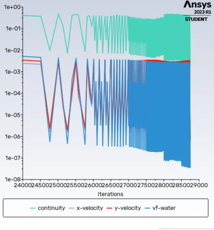
Residual plot :

Animation :

https://drive.google.com/file/d/1zlQVFkBCfDtkkPnefGDVcklWF96gZjkS/view?usp=share_link

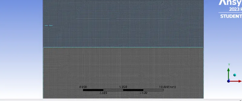
Case 1.1:

MESH	Refined
ELEMENT SIZE	0.15
DENSITY OF PRIMARY FLUID	Air (1.225 kg/m3)
DENSITY OF SECONDARY FLUID	Water (998.2 kg/m3)
ATWOOD NUMBER	0.9975

Residual plot :

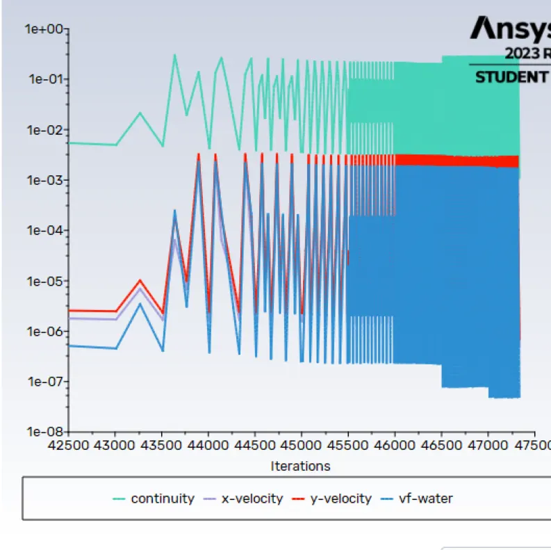
Animation :

https://drive.google.com/file/d/1Ws4Flay2L7Ozp4jQt_n8IWaPGNXnVP6G/view?usp=share_link

Case 2:

The Atwood Number for Water-UD material RT instability

A= (998.2 - 400) / (998.2+400)

we get A=0.427

MESH	Refined
ELEMENT SIZE	0.15
DENSITY OF PRIMARY FLUID	User-defined material (400 kg/m3">m3)
DENSITY OF SECONDARY FLUID	Water (998.2 kg/m3)
ATWOOD NUMBER	0.4278

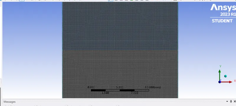
Residual plot :

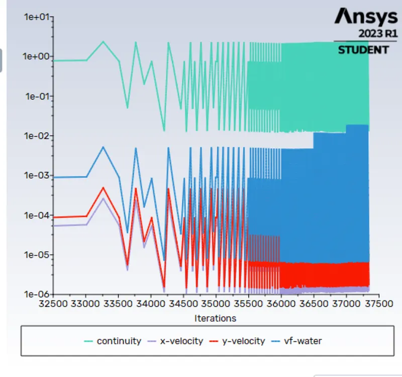
Animation :

https://drive.google.com/file/d/1c-KydasHUAA-5fAwDNeMlARGQffYcYlZ/view?usp=share_link

OBSERVATION :

• The finer mesh captures the instability better than the coarse mesh.but it takes more time for the heavier fluid to settle down.
• The computational time is also increased for fine mesh but the result obtained having better accuracy.
• The steady state simulation is performed if we are concerned more about the final state results or the equilibrium state,In RT instability CFD model we are more concerned to learn about the transition of the irregularities that start developing when we pour the high densiy fluid upon the low density fluid under the effect of gravity and we want to know how the interface collapses as a function of time. so In this case Transient state is more suitable over the steady state.

CONCLUSION :

• It is observed that the more we refine the mesh, the more the simulation results get smoother about the irregularities that take place at the interface of the two fluids. As higher-density fluid replaces lower-density fluid, the formation of air bubbles and vortex takes place, which travels towards the upward region with time.
• In the Rayleigh- Taylor Instability, due to a sudden collapse in the layer between the denser and lighter fluid spike generation takes place which is obviously time-dependent, hence using a steady state solver will not work as we are interested in the flow parameters with respect to time.
• For air- water Atwood number is 0.9975 which is close to 1, so more bubbles is formed which is less symmetrical and also it occurs very rapidly.
• For water- Ud Atwood number is 0.4278 which is close to 0, so bubbles is formed which is relatively symmetrical and the pertubations are linear for larger time.