Week 2 - Flow over a Cylinder.
AIM:
To Simulate the flow over a cylinder and explain the phenomenon of Karman vortex street.
Objective:
1.To Calculate the coefficient of drag and lift over a cylinder by setting the Reynolds number to 10,100,1000,10000 & 100000. (Run with steady solver)
2.Simulate the flow with the steady and unsteady case and calculate the Strouhal Number for Re= 100.
THEORY:
In spite of extensive experimental and numerical studies of almost over a century, flow around a circular cylinder still remains a challenging problem in fluid mechanics, where intensive investigations are continued even today to understand the complex unsteady dynamics of the cylinder wake flow. Cross-flow normal to the axis of a stationary circular cylinder and the associated problems of heat and mass transport are encountered in a
wide variety of engineering applications. Both experimental measurements and numerical computations have confirmed the onset of instability of the wake flow behind a cylinder beyond a critical Reynolds number, leading finally to a kind of periodic flow identified by definite frequencies, well-known in the literature as the Von Karman vortex street. In the case of laminar flow past cylinders with regular polygonal cross-section, the flow
usually separates at one or more sharp corners of the cross-section geometry itself, forming a system of vortices in the wake on either side of the mid symmetry plane. On the other hand, for a circular cylinder, where the point of flow separation is decided by the nature of the upstream boundary layer, the physics of the flow is much more complex than what its relatively simple shape might suggest.
Reynolds Number (Re):
Reynolds number for a flow is a measure of the ratio of inertial to viscous forces in the flow of a fluid around a body.
Re = rho*V*d/Dynamic Viscosity
The range of Re values will vary with the size and shape of the body from which the eddies are being shed, as well as with the kinematic viscosity of the fluid. Over a large Red range (47<Red<105 for circular cylinders; reference length is d: diameter of the circular cylinder) eddies are shed continuously from each side of the circle boundary, forming rows of vortices in its wake. The alternation leads to the core of a vortex in one row being opposite the point midway between two vortex cores in the other row, giving rise to the distinctive pattern shown in the picture. Ultimately, the energy of the vortices is consumed by viscosity as they move further downstream, and the regular pattern disappears.
Strouhal number (St):
Strouhal number is a dimensionless number describing oscillating flow mechanisms.
The Strouhal number is often given as
St = f*d/u
Where,
f is the frequency of vortex shading,
L is the characteristic length and
U is the flow velocity.
Procedure:
Geometry:
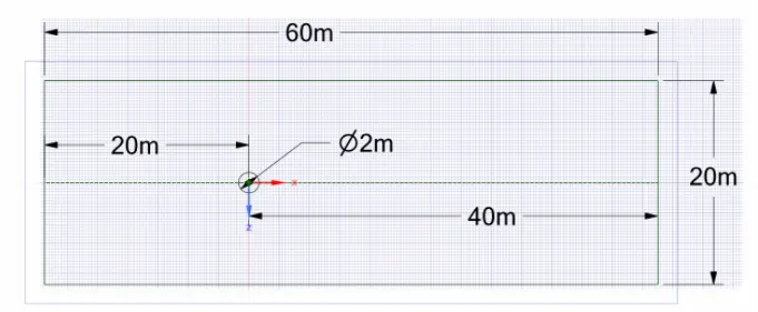
A plate with the dimension of 20*60m is created using spaceclaim.
Meshing:
1.Now select the body and go to mesh and click on generate mesh with mesh size 0.25 m.To ensure triangular mesh, go to mesh > insert > select triangular mesh type.
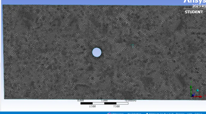
2.After generating mesh,it is seen that size of cirle looks distoreted.
go to mesh > sizing > select circular edge > deffinition >type > no,of divisions >36.
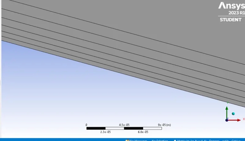
3.To capture better results near cylinder wall, go to mesh > inflation > select the body and edge > inflation option : 1st layer thickness >1 st layer height :5e-3 m >maximum layer :6
4..select the edges of geometry and named them as inlet,outlet ,wall and symmetry.
PART 1:
REYNOLDS NUMBER:
For Re = 100:
Re=U⋅ρ⋅Dμ">Re=U⋅ρ⋅D/μ
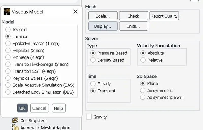
velocity = 1 m/s.
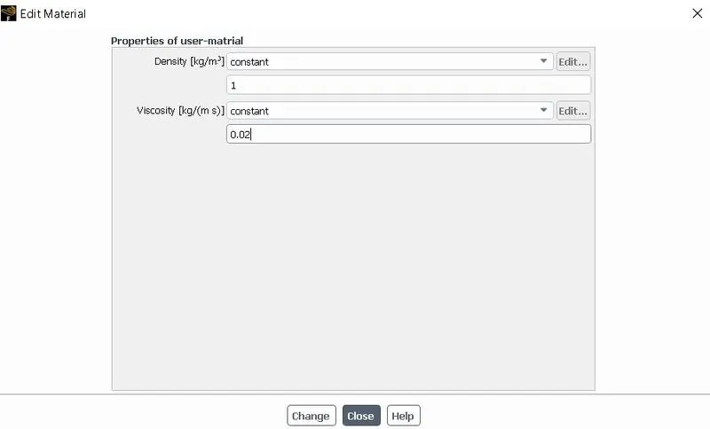
density = 1 kg/m3.
viscosity = 0.02 kg/ms.
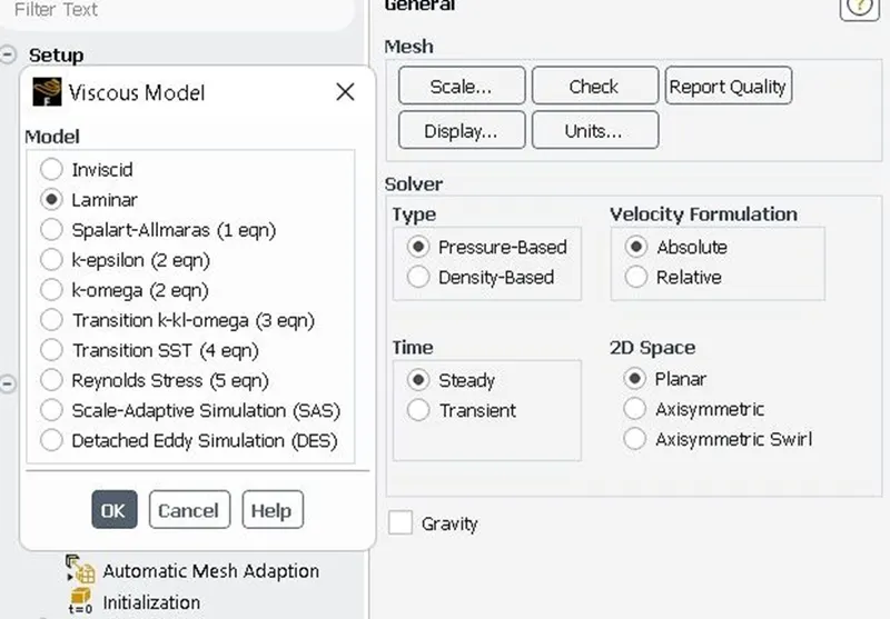
STEADY STATE :
UNSTEADY STATE :
Material :
Cell zones :
BOUNDARIES :
Inlet (velocity inlet) Velocity magnitude 1m/s
- Outlet (pressure outlet) Gauge pressure – 0 pa
- Symmetry – symmetry
- Walls – stationary wal
Condition - No slip
SOLUTION:
- Vertex average of velocity magnitude using surface report at a monitor point at 10m from the center of the cylinder to the right of the cylinder along the x-direction.
- Coefficient of drag and coefficient of lift reports are created using force report
INITIALIZATION: Hybrid for steady state
The standard for unsteady state
ACTIVITIES: contour plots of pressure and velocity and solution animation are created after initialize the solution.
RUN CALCULATION:
For steady-state – No of iterations= 500
For transient state – Time step = 0.1
No of iterations = 500
RESULTS:
STEADY-STATE:
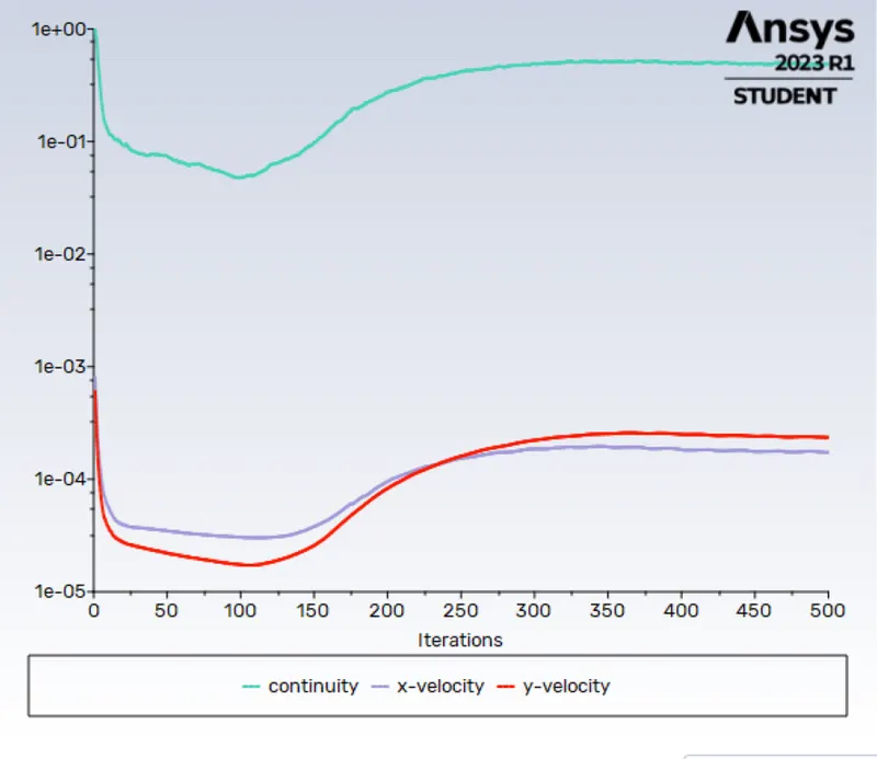
RESIDUAL:
This plot helps in monitoring the change in each and every convergence criterion for every time step and plots those values for every iteration or time step. This plot helps to know when convergence is achieved.
MONITOR POINT VELOCITY:
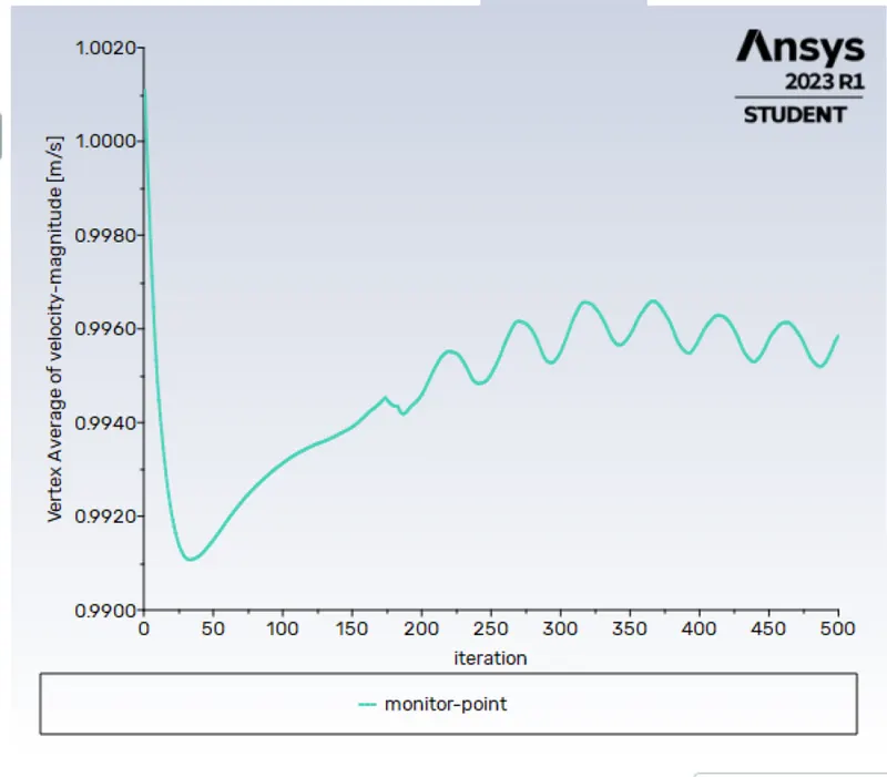
The above plot shows the value of vertex average of velocity magnitude at the monitor point is 0.9958491 m/s
CONTOUR:
VELOCITY:
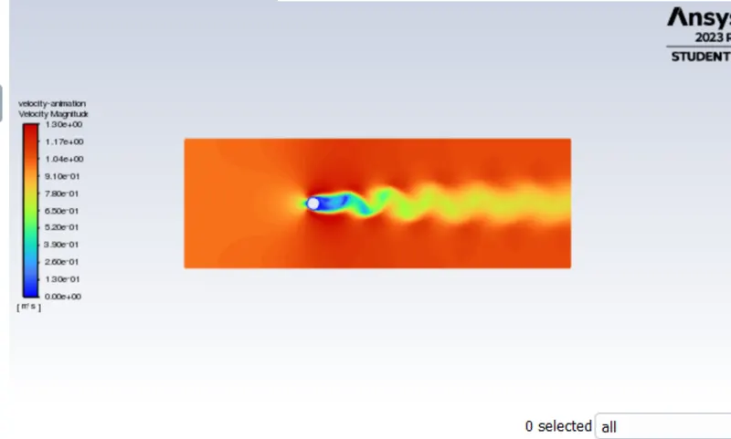
ANIMATION LINK :
https://drive.google.com/file/d/1D7jM6PxowbKo2au1fwiV-SyKM7_lw8KN/view?usp=share_link
PRESSURE:
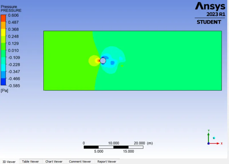
ANIMATION LINK :
https://drive.google.com/file/d/1Z14CA0lKGGu9hXy340hF3qv0OxR-2p4r/view?usp=share_link
DRAG PLOT:
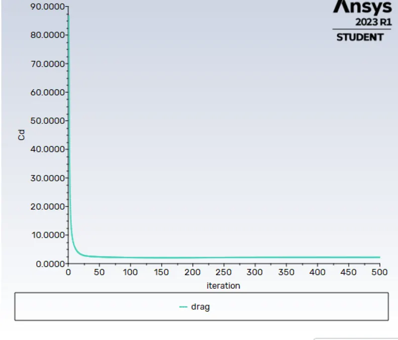
The coefficient of the drag plot shows the constant value after a certain number of iterations and remains the same after that and the value is 1.3403629
LIFT PLOT:
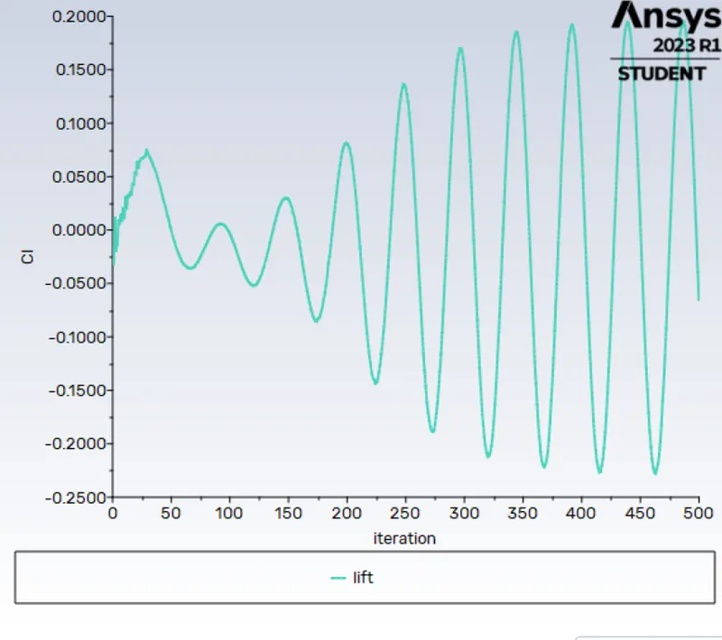
The coefficient of the lift plot shows that it starts oscillating after some time and continues further and the value is 0.179.
STROHAUL NUMBER:
The strohaul number cannot be calculated for the steady state as we don't calculate the flow with respect to time
TRANSIENT:
RESIDUAL:
This plot helps in monitoring the change in each and every convergence criterion for every time step and plots those values for every iteration or time step. This plot helps to know when convergence is achieved.
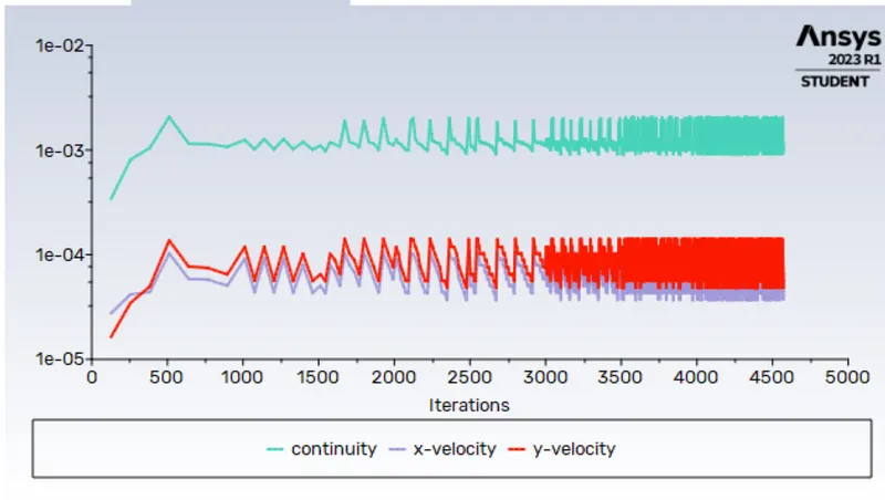
The flow is converged in 4600 iterations.
MONITOR POINT VELOCITY:
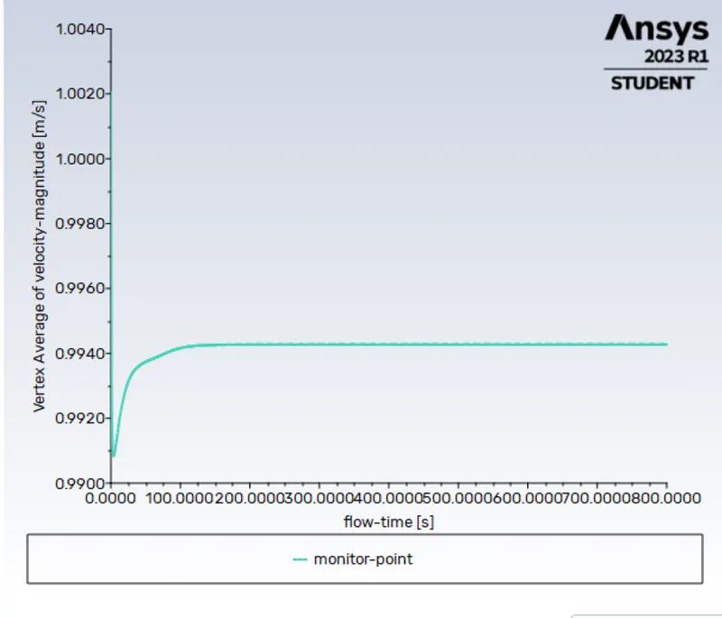
The above plot shows the value of vertex average of velocity magnitude at the monitor point is 0.9823 m/s
CONTOUR:
VELOCITY:
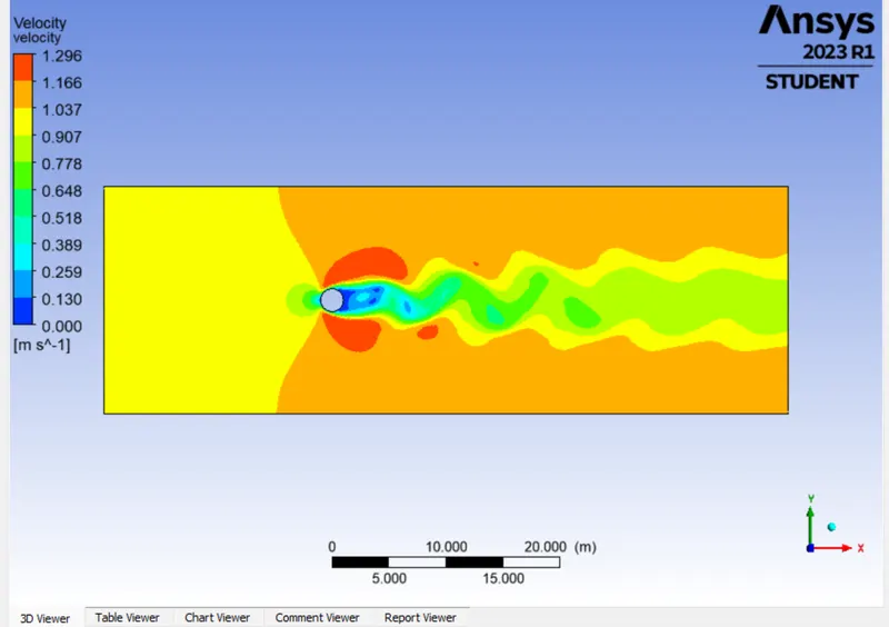
PRESSURE:
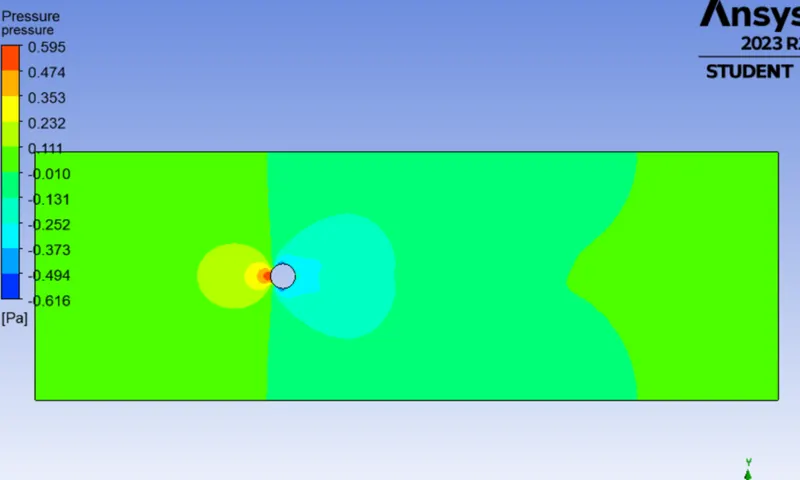
DRAG PLOT:
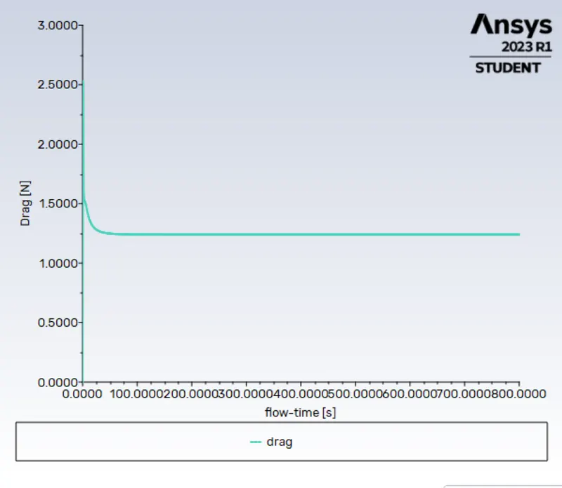
The coefficient of the drag plot shows the constant value after a certain number of iterations and remains the same after that and the value is 1.2403638
LIFT PLOT:
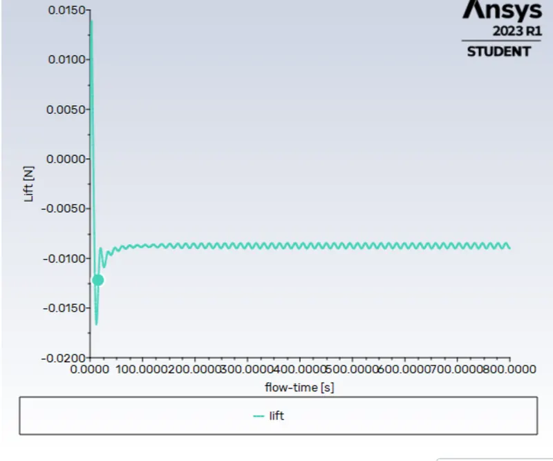
The coefficient of the lift plot shows that it starts oscillating after some time and continues further and the value is -0.014673849
STROHAUL NUMBER:
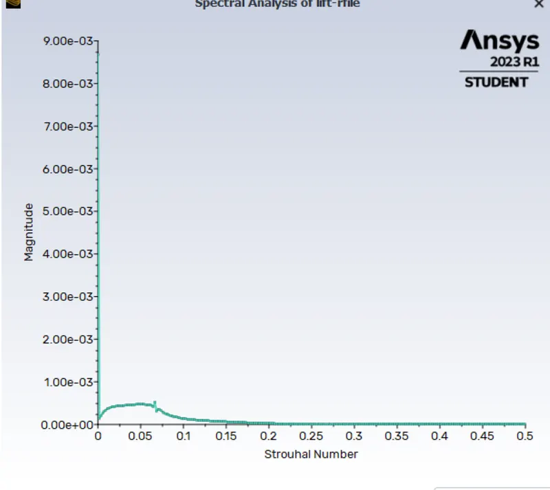
Strohaul number = 0.01.
SUMMARY:
| CASES | REYNOLDS NUMBER | INLET VELOCITY | Cd | Cl | MONITOR VELOCITY |
| STEADY STATE | 100 | 1m/s | 1.3403629 | 0.17997243 | 0.9958491m/s |
| TRANSIENT STATE | 100 | 1m/s | 1.2403638 | -0.014673849 | 0.9823 m/s |
From the above cases, we can say that in the transient case the velocity starts oscillating for the monitoring point after certain iterations and the velocity at the monitoring point is greater in the case of the steady-state case as compared to the transient case.
SIMULATION OF FLOW FOR THE STEADY STATE FOR Re = 10
Velocity calculation for Reynolds number 10,
For Re = 10:
RESULTS:
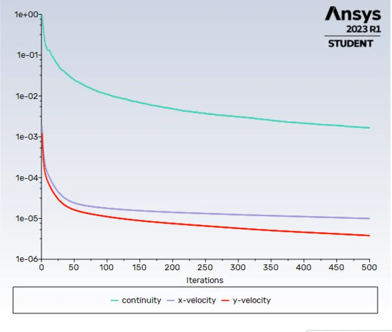
RESIDUAL:
This plot helps in monitoring the change in each and every convergence criterion for every time step and plots those values for every iteration or time step. This plot helps to know when convergence is achieved.
MONITOR POINT VELOCITY:
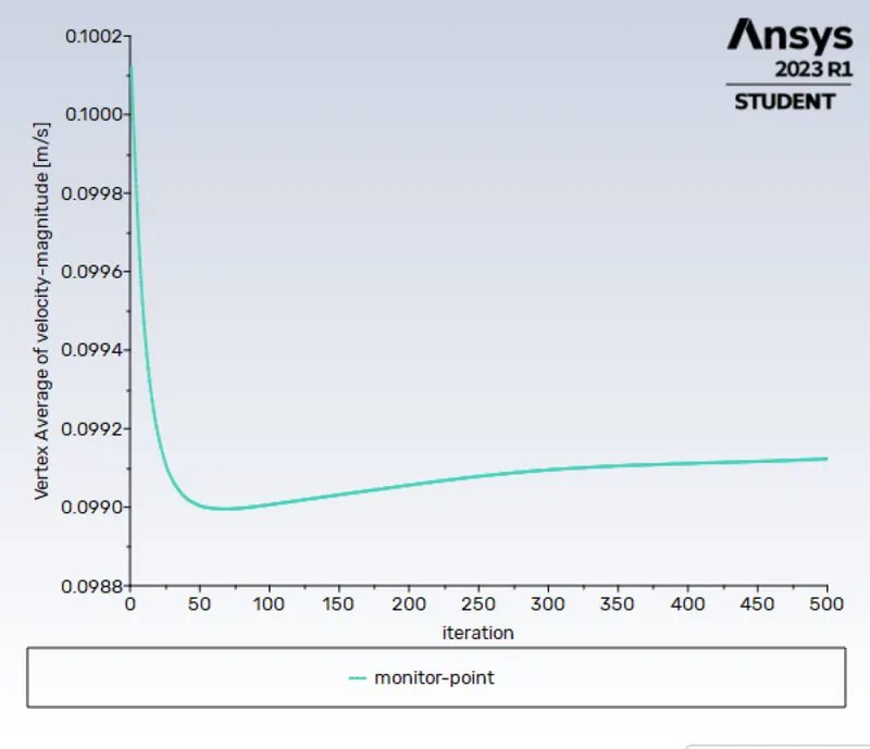
From this plot we can see that for re = 10 ,0.09912314
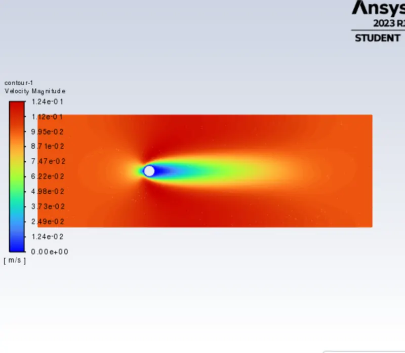
CONTOUR:
VELOCITY:
DRAG PLOT:
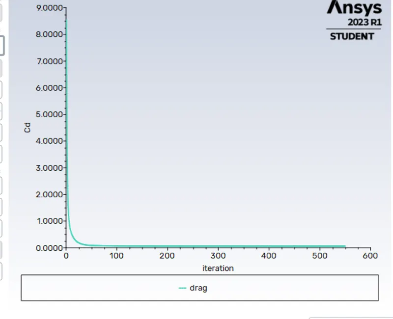
The coefficient of the drag plot shows the constant value after a certain number of iterations and remains the same after that and the value is 3.3314425
LIFT PLOT:
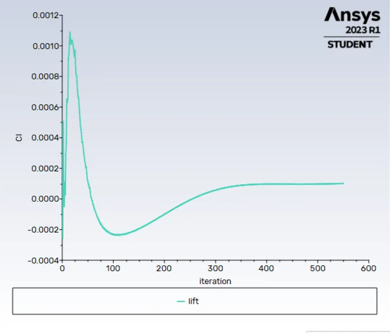
The coefficient of the lift plot shows that it starts oscillating after some time and continues further and the value is 0.000101008
SIMULATION OF FLOW FOR THE STEADY STATE FOR Re = 100
Velocity calculation for Reynolds number 100,
For Re = 100:
Re=U⋅ρ⋅Dμ">Re=U⋅ρ⋅D/μ
100=U.1.2/0.02
U=1m/s
RESIDUAL:
This plot helps in monitoring the change in each and every convergence criterion for every time step and plots those values for every iteration or time step. This plot helps to know when convergence is achieved.
MONITOR POINT VELOCITY:
The above plot shows the value of vertex average of velocity magnitude at the monitor point is 0.9958491 m/s
CONTOUR:
VELOCITY:
ANIMATION LINK :
https://drive.google.com/file/d/1D7jM6PxowbKo2au1fwiV-SyKM7_lw8KN/view?usp=share_link
DRAG PLOT:
The coefficient of the drag plot shows the constant value after a certain number of iterations and remains the same after that and the value is 1.3403629
LIFT PLOT:
The coefficient of the lift plot shows that it starts oscillating after some time and continues further and the value is 0.179.
SIMULATION OF FLOW FOR THE STEADY STATE FOR Re = 1000
Velocity calculation for Reynolds number 1000,
For Re = 1000:
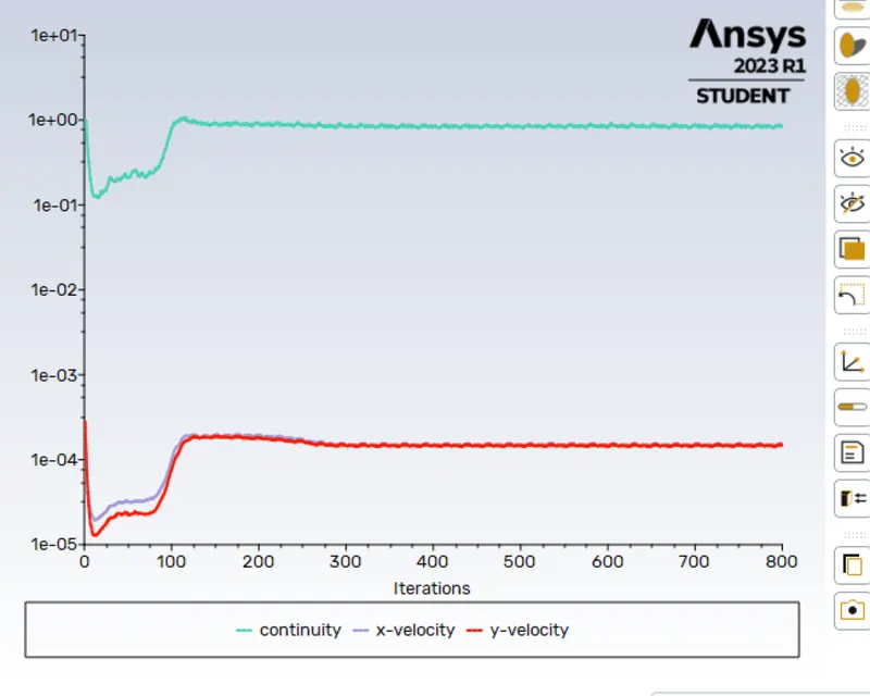
RESIDUAL:
MONITOR POINT VELOCITY:
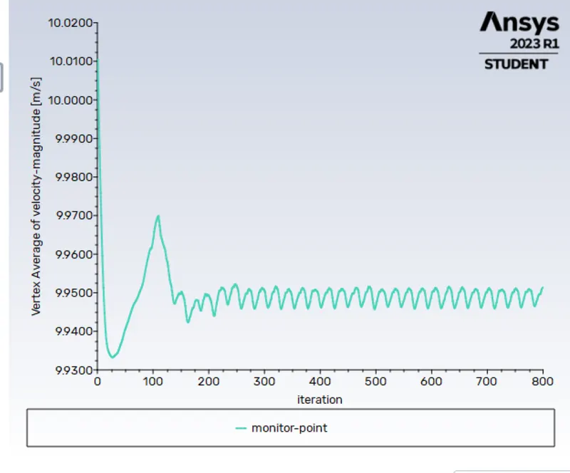
The above plot shows the value of vertex average of velocity magnitude at the monitor point is 9.951334 m/s
CONTOUR:
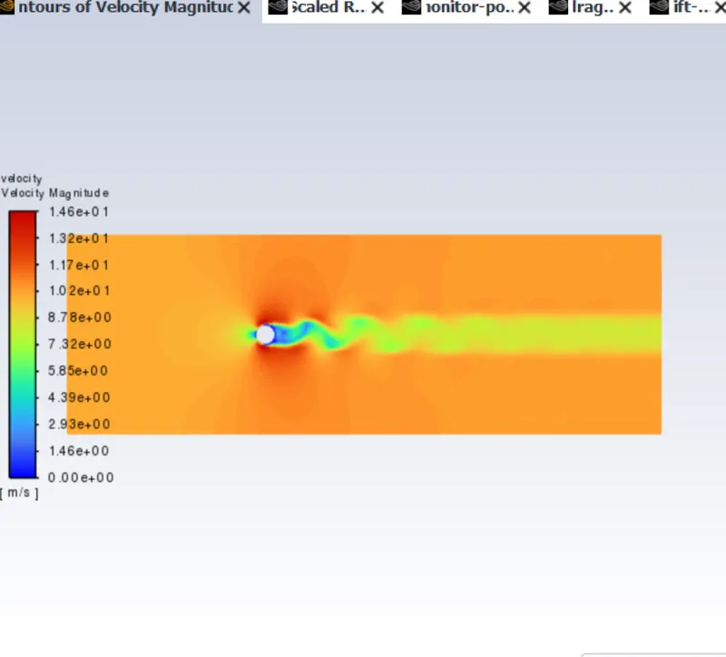
VELOCITY:
DRAG PLOT:
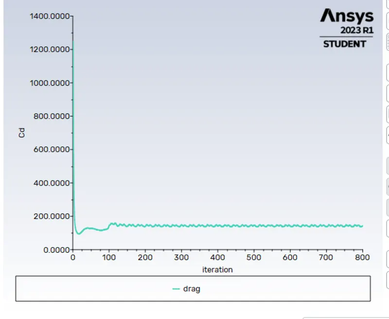
The coefficient of the drag plot shows the constant value after a certain number of iterations and remains the same after that and the value is 0.969124.
LIFT PLOT:
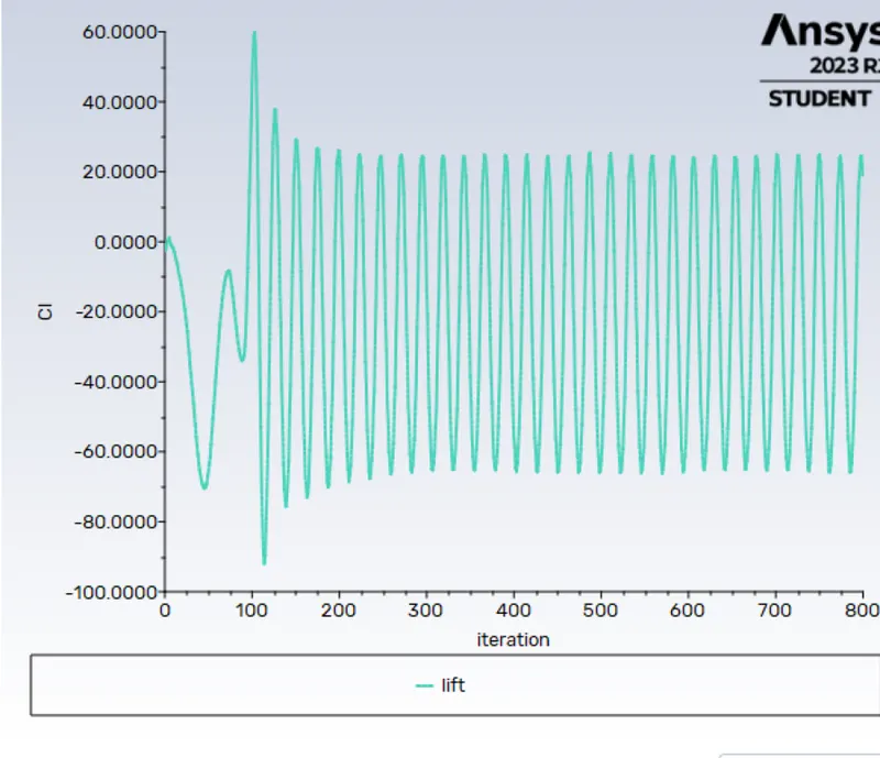
The coefficient of the lift plot shows that it starts oscillating after some time and continues further and the value is -0.4399
SIMULATION OF FLOW FOR THE STEADY STATE FOR Re = 10000
Velocity calculation for Reynolds number 10000,
For Re = 10000:
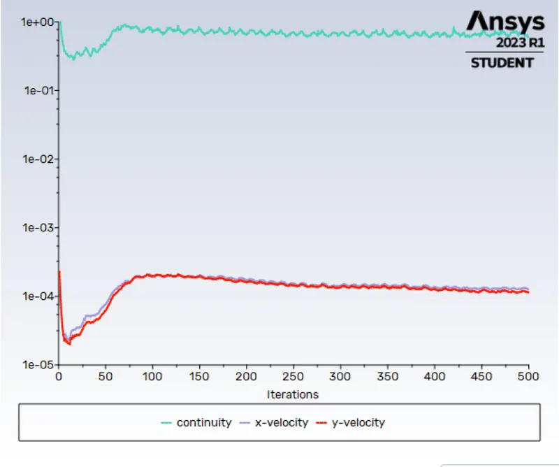
RESIDUAL:
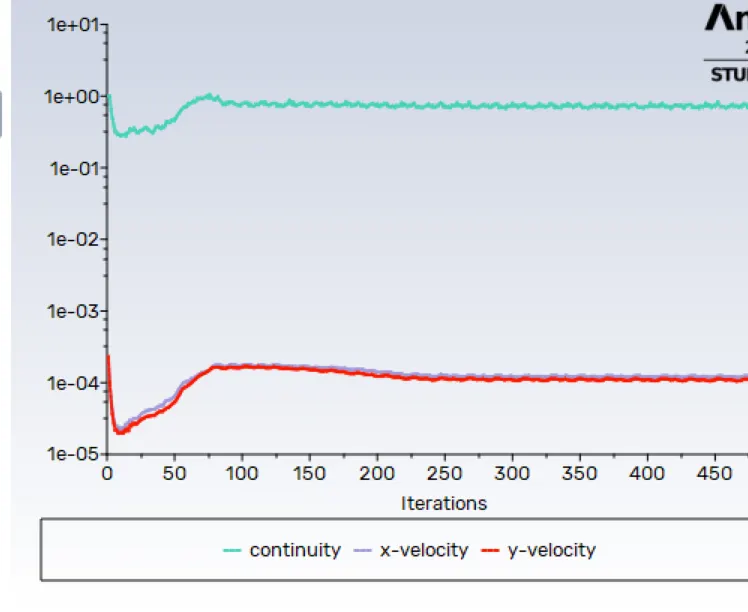
MONITOR POINT VELOCITY:
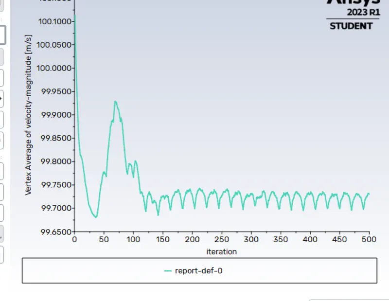
The above plot shows the value of vertex average of velocity magnitude at the monitor point is 99.73012 m/s
CONTOUR:
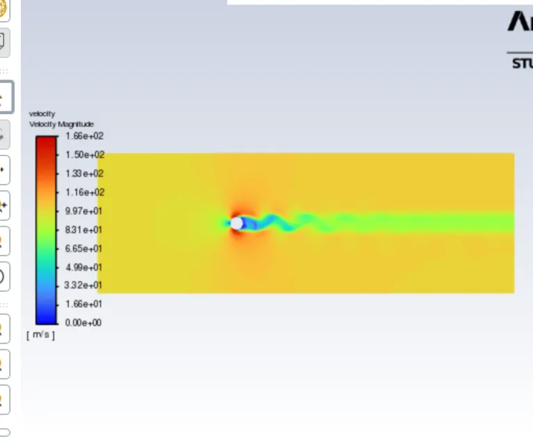
VELOCITY:
DRAG PLOT:
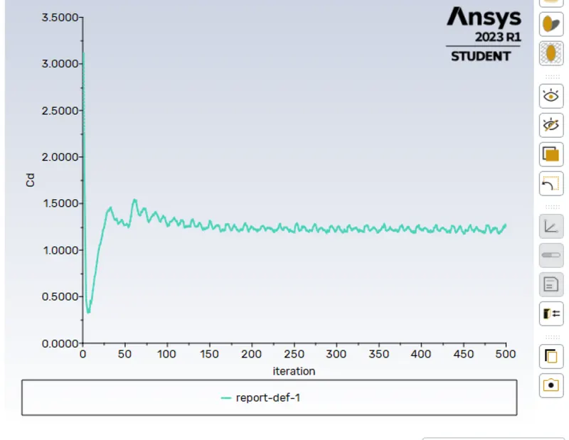
The coefficient of the drag plot shows the constant value after a certain number of iterations and remains the same after that and the value is 0.869121
LIFT PLOT:
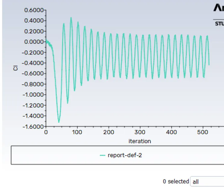
The coefficient of the lift plot shows that it starts oscillating after some time and continues further and the value is -0.94516
SIMULATION OF FLOW FOR THE STEADY STATE FOR Re = 100000
Velocity calculation for Reynolds number 100000,
For Re = 100000:
RESIDUAL:
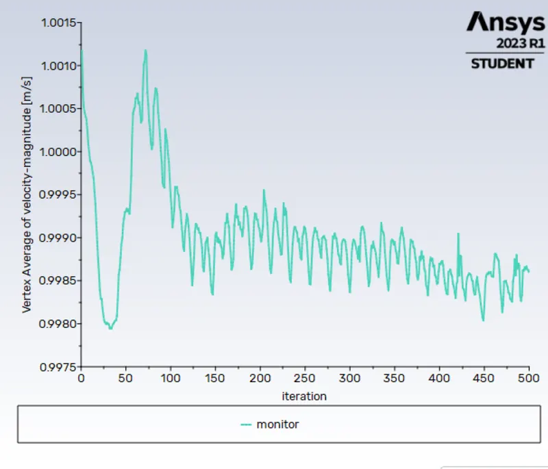
MONITOR POINT VELOCITY:
CONTOUR:
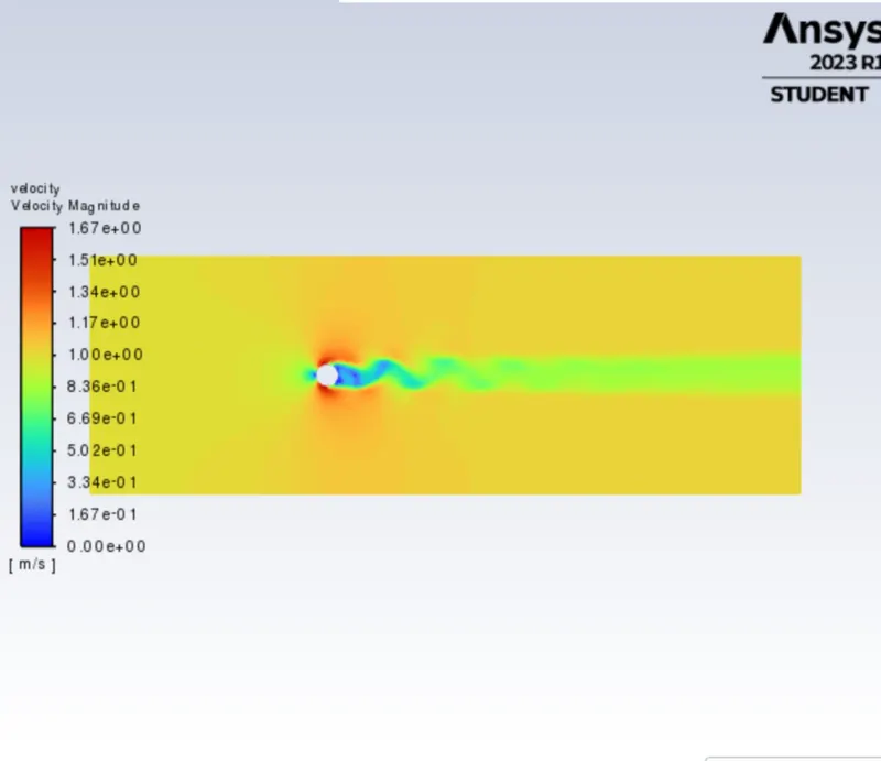
VELOCITY:
DRAG PLOT:
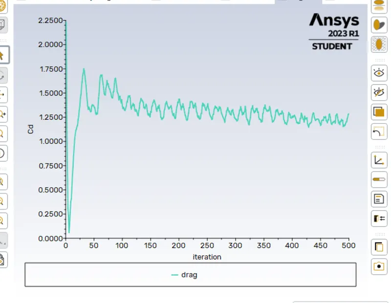
The coefficient of the drag plot shows the constant value after a certain number of iterations and remains the same after that and the value is 0.64184392
LIFT PLOT:
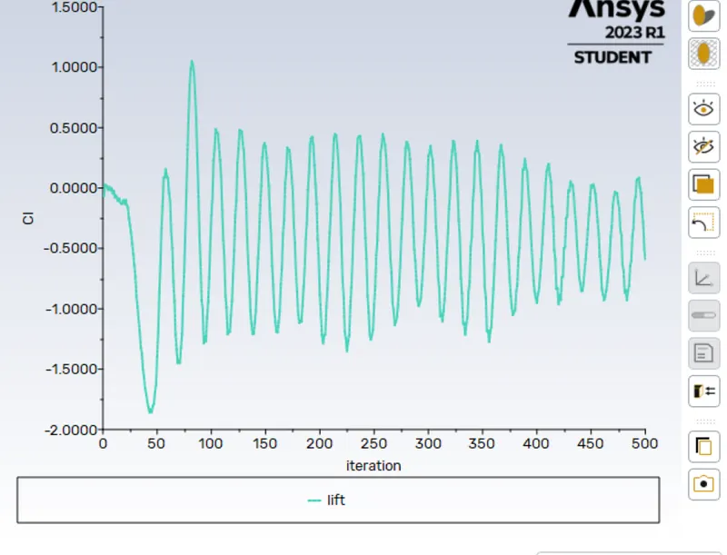
The coefficient of the lift plot shows that it starts oscillating after some time and continues further and the value is -0.29432254
SUMMARY:
| SIMULATION | REYNOLDS NUMBER | Cd | Cl |
| 1 | 10 | 3.3314425 | 0.000101008 |
| 2 | 100 | 1.3403629 | 0.17997243 |
| 3 | 1000 | 0.969124. | -0.4399 |
| 4 | 10000 | 0.869121 | -0.94516 |
| 5 | 100000 | 0.64184392 | -0.29432254 |
From the above plot, we can say that the value of the lift coefficient keeps on increasing as we keep increasing the velocity and Reynolds number. The drag coefficient is maximum for the lowest Reynolds number and goes on decreasing.
CONCLUSION:
- When fluid flows over the cylinder, the wake region is formed next to the cylinder due to a decrease in pressure, and recirculation of flow occurs hence flow separation occurs.
- As flow over a cylinder is transient we are unable to observe flow separation at a low Reynolds number
- As the Reynolds number increases the coefficient of drag decreases.
- Strauhal number for an unsteady state with Reynolds number 100 is 0.01.