Week 4 - CHT Analysis on Exhaust port

AIM:

The aim of this project is to simulate the conjugate heat transfer simulation inside an exhaust manifold.

Objectives:

• Brief description of where and why CHT analysis is used
• Maintain the Y+ value according to the turbulence model and justify the results
• Wall and surface heat transfer coefficient on the internal solid surface and the velocity and temperature contours in the appropriate areas
• Verification of the HTC from the simulations and factors on which its accuracy depends

INTRODUCTION:

Heat transfer problems can be considered into the various aspects like conjugate, coupled or adjoint simulation. These terms corresponds to the problems consisting of two or more subdomains based on distinct differential equations depending upon the method used. The heat transfer between a body and a fluid flowing past it, is a conjugate type of problem, because the heat transfer inside the body is governed by the elliptical Laplace equation or by the parabolic differential equation, whereas the heat transfer inside the fluid is governed by the elliptical Navier-Stokes equation or a parabolic boundary layer equation. The solution of such problem gives the temperature and heat flux distributions on the interface. Thus the CHT is the situation where a solid and fluid interacts with each other and we need to know the thermal exchange at the interface or within the solids and fluids. One of the example of it can be hot or cold air moving past a solid body and resulting to the change in its temperature.

THEORY :

CHT analysis can be performed to improve the cooling of the water jacket and improve the engine life among many other applications. Critical cooling applications most of the time depends on multiple thermal protection techniques, like internal, external film cooling, etc. which are efficiently used in our analysis to cool components and limit the use of coolant.

The below listed models are generally used to turbulence modelling because of the need of additional equations for making the problem closed.

Spalart-allmaras model is 1 equation model, which are developed and used extensively for aerospace industry application. On the other hand k- omega and k- epsilon are two equation models. These are semi-analytic models by the way. k- Epsilon model predicts far from the boundaries (wall) & k- omega model predicts well near wall. Even though it depends on Y+. We also have SST model which is a combination of these. Selection of model depends on the specific problem, no turbulence model is suited for the every case. Fine tuning is required. SST model used good mesh at boundary and with wall treated usually works in most cases, but again it is problem specific and we need to do the analysis of different kind and with different physics for all the cases which suits it. In this particular steady state simulation we are going to analyse the simulation through an exhaust port with total four inlets coming from the 4 cylinder engine and then resulting into a single port of exhaust outlet. The velocity and temperature variations among the different solid sections and inside the intricate shapes of the exhaust port needs to be shown to have better understanding of the flow characteristics with respect to its fluid section and the boundary layers.

EXHAUST PORT SIMULATION(BASE LINE MESH)

The stages involved in the simulation are as follows

• Geometry
• Mesh
• Setup
• Solution
• Results

Geometry :

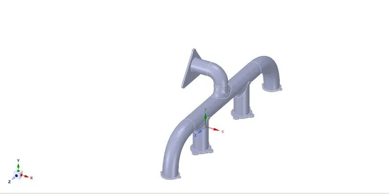
He first step is to import the geometry into spaceclaim and extract the fluid volume where the fluid interacts with the exhaust port for 4 cylinder inline engine.

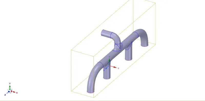
Now we show the image where we have created the fluid volume and now we have to enable the share topology.

Mesh :

Case 1:

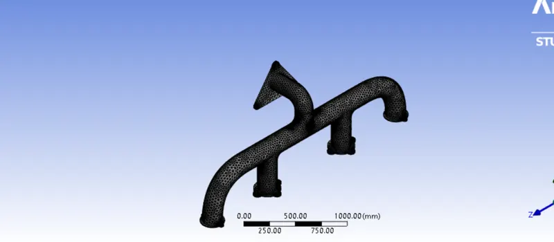
Base line mesh with element size 150mm with no inflation layer also with 138040 elements

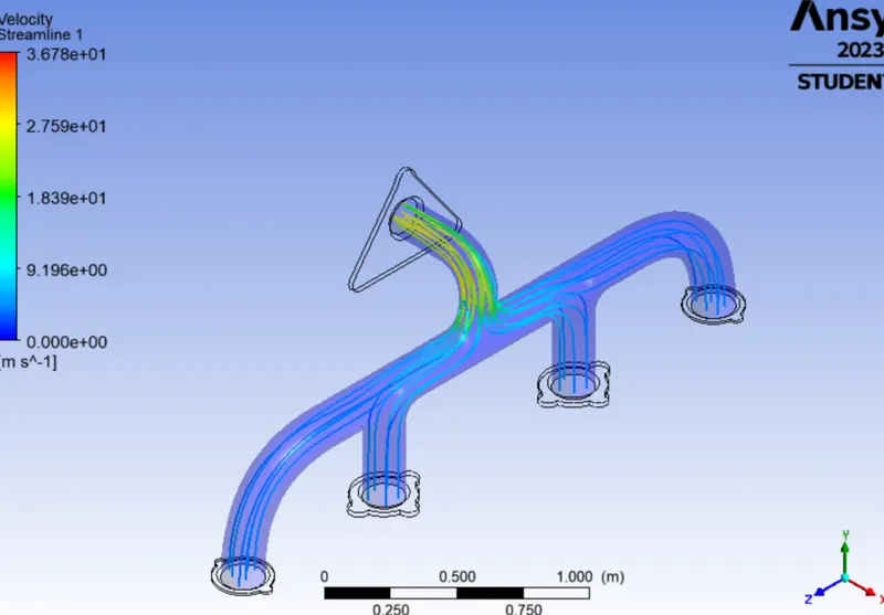
Solver Settings – Ansys Fluent was used as the solver and steady state simulations have been performed using a density based solver. Air was used as the fluid. The inlet velocity was 5 m/s at 700 K.

Material	Density(kg/m^3)	Specific heat(J/kg-K)	Thermal Conductivity(W/m-K)	Viscosity(kg/m-s)
Fluid (AIR)	1.225	1006.43	0.0242	1.7894e-05
Solid (Aluminium)	2719	871	202.4	---

BOUNDARY CONDTIONS:

At inlet the temperature of air is maintained at 700K and such all 4 inlets are taken into considerations through which the exhaust air with an absolute velocity of 5m/sec is considered to flow through.At outlet the pressure is assumed to be at atmospheric pressure and thus the gauge pressure is maintained at 0 Pa only and the velocity and temperature has to be analysed later in post processing.Outer wall convection which have the convective heat transfer coefficient as 20W/m^2-K and the free stream temperature of around 700K.

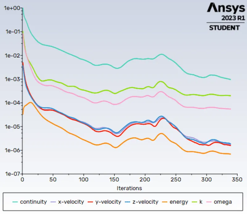
Residuals:

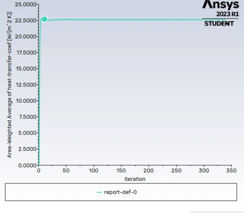
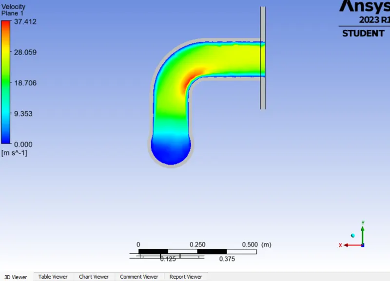
velocity plane plot :

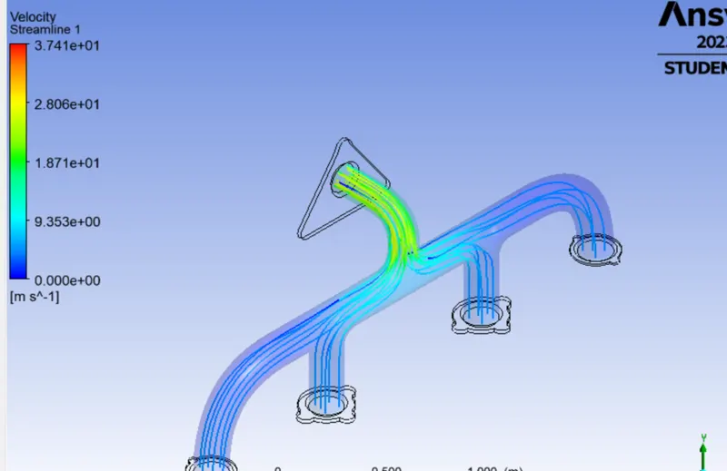
velocity streamline :

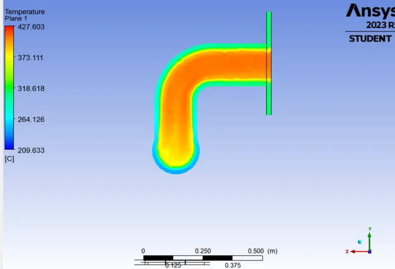
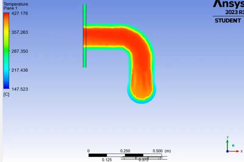
Temperature plane plot :

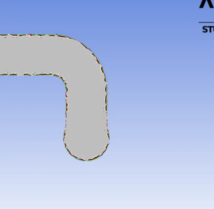
Wall heat tranfer coefficient plot:

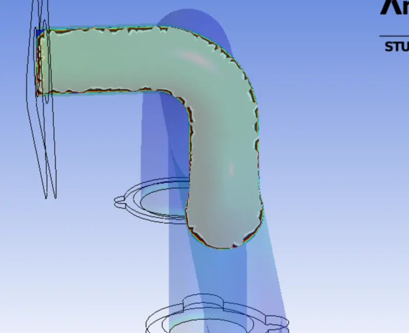
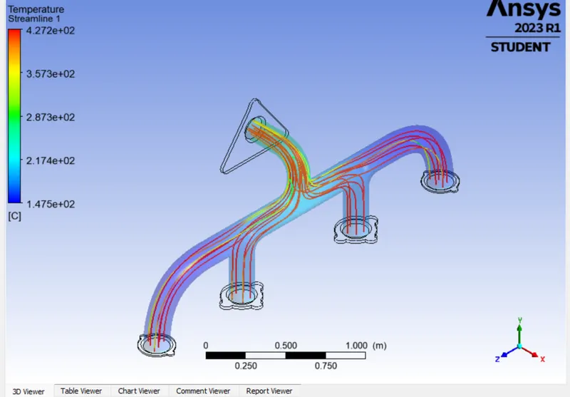
Temperature streamline :

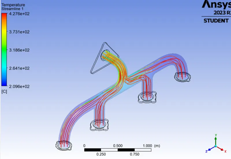
As the base line mesh doesn't have infation layer catching the wall heat transfer coefficient will not be accurate.So inorder to catch the phenomenons near the wall condition the best choice is to construct an inflation layer and Use k-omega SST turbulance model.Combination of these along with proper y plus value we can get near to the experimental value.

case 2:

Refined mesh with Inflation layer:

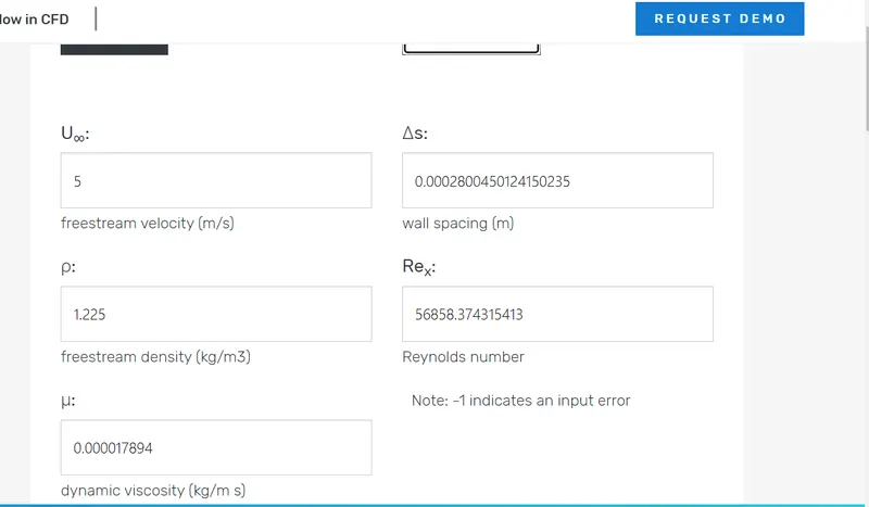
The refined mesh with element size 200mm altogether with inflation layer determined by hand calculating y plus value as 0.00028m.The refined mesh has 257847 elements.Further details are shown below.

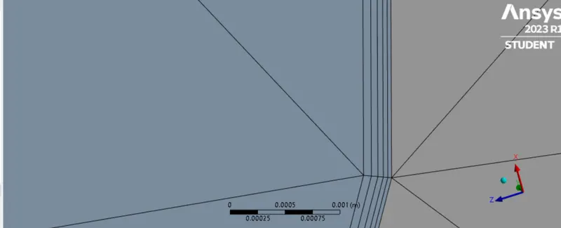
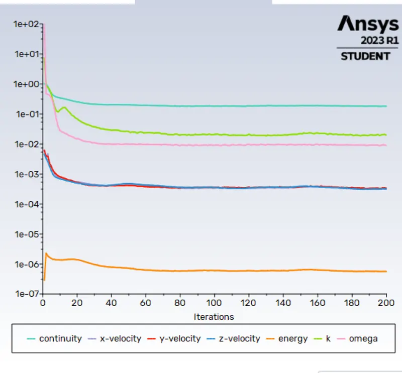
Residuals:

velocity plane plot :

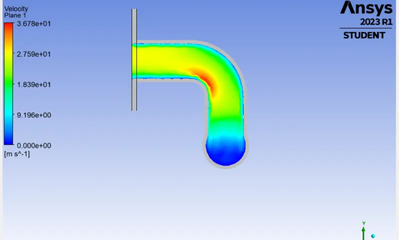
velocity streamline :

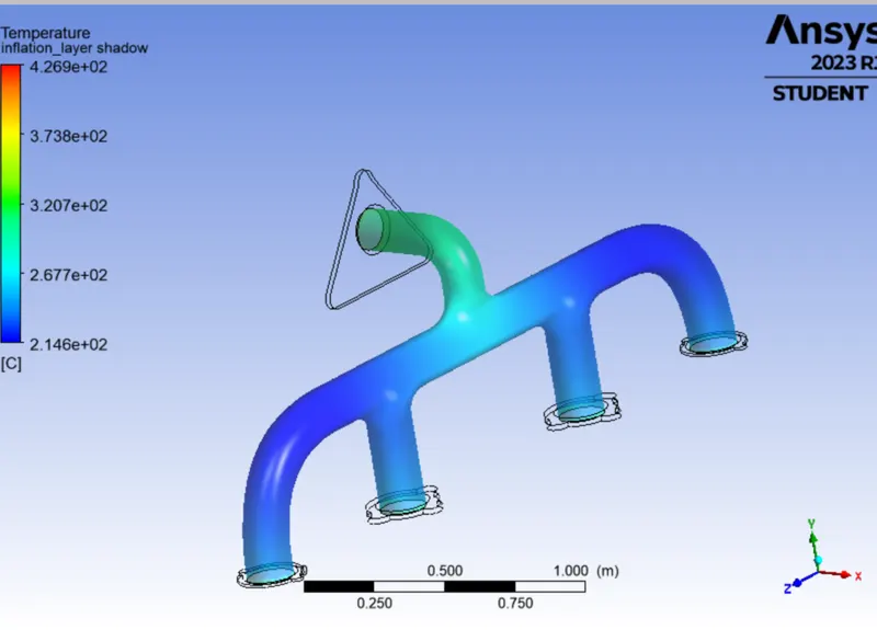
Temperature plane plot :

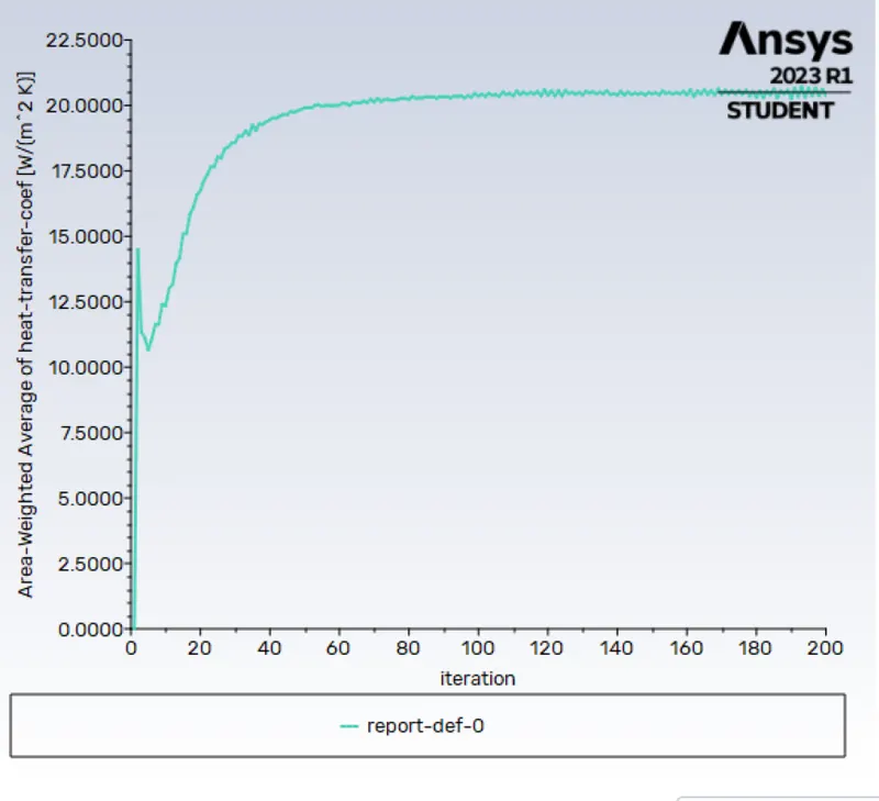
Wall heat tranfer coefficient plot:

Temperature streamline :

To verify the simulations are correct we need to hand calculate the thermal or heat tranfer coefficient.

Nu=0.023.Re^4/5.Pr^n

• Nu = Nusselt No.
• Re = Reynolds No.
• Pr = Prandtl No.
• n = Heating Component = 0.4

Nusselt Number = Nusselt number is defined as the ratio of convection heat transfer to conduction heat transfer across a boundary in a fluid

Nu = hD/k

• h = Heat transfer coefficient
• D = Hydraulic Diameter
• k =Thermal Conductivity of Fluid i.e Air

Prandtl Number= It is defined as the ratio of momentum diffusivity to thermal diffusivity

Pr = µCp/k

µ = Dynamic Viscosity

Cp = Specific Heat Capacity

k = Thermal Conductivity of Fluid i.e Air

Now For 700 Kelvin( which is our temperature value for the simulation)

Cp = 1.0750 Kj/Kg-K

Pr = 0.71

µ = 1.7894 E - 5 kg/m-s

Reynolds Number = 56858.37

Putting the values in Dittus-Boelter Equation Nusselt No comes out to be 127.66

Diameter = 0.16611 meters

Thermal Conductivity = 0.026 W/mK

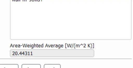
From There The Value of Heat Transfer Coefficient comes out to be 20 W/(m^2 K)

The heat transfer coefficient value from simulation results 20.44 W/(m^2 K)

The Accuracy of Predictions Depends on several factors like:

Clean geometry:removing interferences and open edges are one amoung the top priority

refinning mesh: The finer the mesh the closer the simulated value gets to experimental value.

Solver type:Choosing correct solver

Viscous model:Choosing the correct turbulance model for example k-omega SST is chosen over k-epsilon because it can catch Boundary phenomenons better than k -epsilon.

Y plus value:the y plus range should be according to the visous model the user choose

other factors like convegance, Number of iterations,Boundary conditions etc.

Conclusion

From the base line mesh which doesn't have inflation layer and from the Refined mesh we can conclude that The model with inflation layer can trap better wall adjacent values and conditions.Also means that inflation layer is needed to capture near wall phenomenons.

As a fact we know that finer the mesh accurate the values are.The viscous models and solvers should be chosen according to the requirements.A good understanding of solvers and models are needed for CHT analysis.Y plus values should be maintained depending on the solvers.Comparing the contours of temperature between the base line mesh and refined mesh we have seen that temperature is more accurate in refined