Week 5 - Rayleigh Taylor Instability

Aim : To Perform Rayleigh Taylor Instability Simulation

Objective : To Perform Rayleigh Taylor Instability Simulation with

1. air and water with base mesh size as 0.5 mm and with refined mesh.
2. water and user defined material(density = 400 kg/m³, viscosity = 0.001 kg/m-s) with refined mesh.

Theory : Rayleigh Taylor occurs whenever a fluid of higher density penetrates a fluid of lower density with acceleration or gravity. The heavier fluid tends to sink down, and the lighter fluid will rise up, causing distortion at the interface.Small initial penetrations will grow into spikes, which will eventually dissolve in a mushroom pattern.The turbulent mixing of fluids also takes the form of a cosine wave.

1. What are some practical CFD models that have been based on the mathematical analysis of Rayleigh Taylor waves? In your own words, explain how these mathematical models have been adapted for CFD calculations.

The practical CFD Models that have been based on the mathematical analysis of Rayleigh Taylor Waves are as follows

• Kelvin-Helmholtz instability
• Richtmyer-Meshkov instability
• Plateau-Rayleigh instability

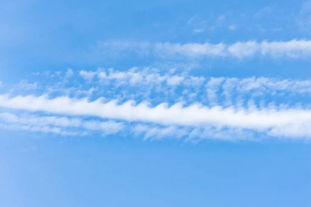
Kelvin-Helmholtz Instability :

• The phenomenon occurs between two immiscible fluids whenever there is a velocity difference at the interface of fluid.
• The instability can be seen between a cloud and the surrounding air.

Richtmyer-Meshkov Instability :

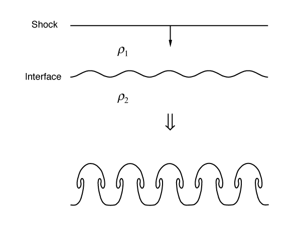
• It is the fluid flow phenomena that occurs when a shock wave strikes an interface separating two gases with varying densities (in the normal direction).
• The instability causes perturbations at the interface to increase, resulting in vortical structures that could lead to a turbulent mixing layer.

Plateau-Rayleigh Instability

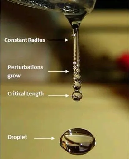
• Energy is required to increase the surface area, and for the same volume of a liquid, the spherical shape has a lower surface area when compared with a cylinderical shape,so in return, the water is trying to minimise its surface area, and its shape changes from cylinderical to spherical. As a result of that, we are able to see a wavy pattern known as Plateau-Rayleigh Instability.
• The phenomenon is happening mainly due to the surface tension of the water.
• Example : Water falling from a jet

Mathematical Models that have been adapted for CFD calculations are as follows

• Mass Diffusion Model
• Single Fluid Model

• Potential Flow Model
• Buoyancy Drag Model
• Besnard-Harlow-Rauenzahn(BHR) Model

• Multi Fluid Model

• Two equation K-L turbulence model
• Three equation K-L-a turbulence model
• Four equation K-L-a-b turbulence model

Why a steady-state approach might not be suitable for these types of simulation

Steady State Approach is not suitable for these types of simulations as steady state approach is time independent and in our simulations we need to study the time dependent physics of turbulent mixing nature of two fluids which is frequently changing with respect to time.

2. To Perform the Rayleigh Taylor instability simulation for 2 different mesh sizes with the base mesh being 0.5 mm

Geometry Preparation

• Create two squares of dimension (20X20 mm) with upper square representing as water(heavier component) and bottom square as air ( lighter component)
• Converted them into surfaces using Pull Tool

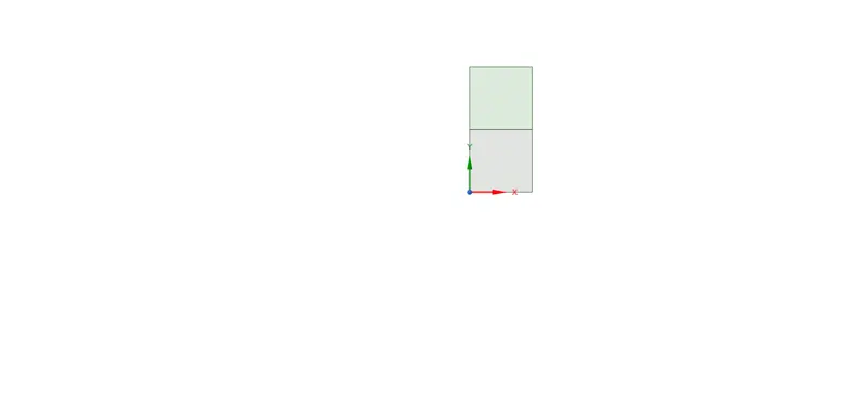
• Sharing Topology

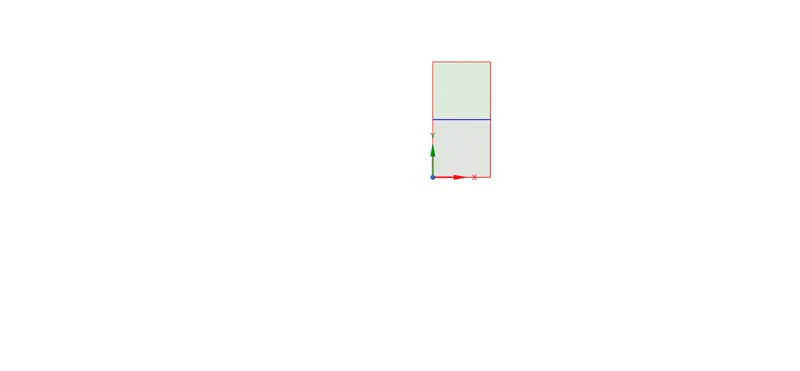
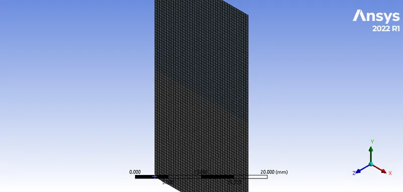
Case1 Meshing The Geometry for Base Line Simulation( i.e mesh size = 0.5 mm)

Setup

• Solver Type : Pressure Based
• Solver Time : Transient
• Gravity : -9.81 m/s^2 (downward y direction)
• Viscous Model -> Laminar
• Multi-Phase-Model

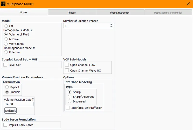
• Primary and Secondary phase (i.e air and water)

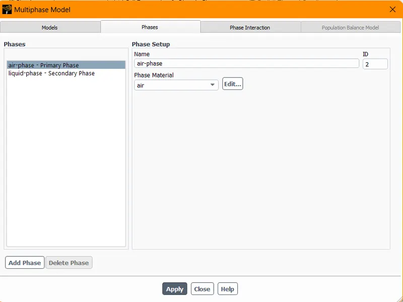
• Formulation -> Implicit Type
• Materials Selection

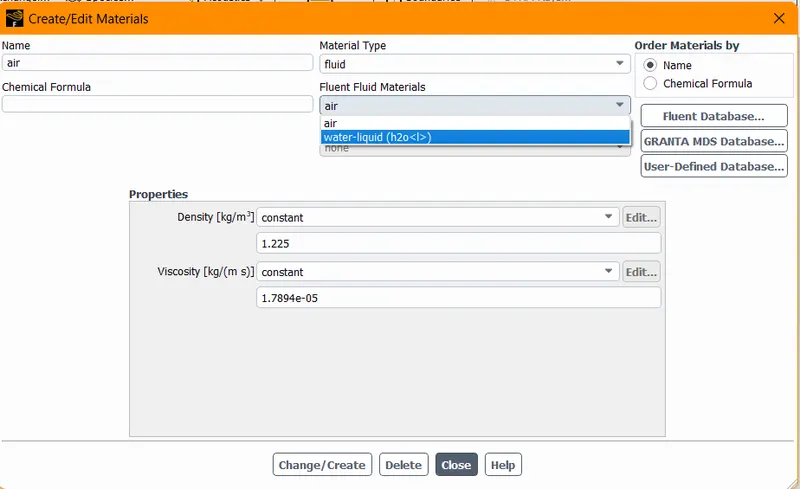
• Patch -> Volume-Fraction -> Water -> 1 -> Air -> 0

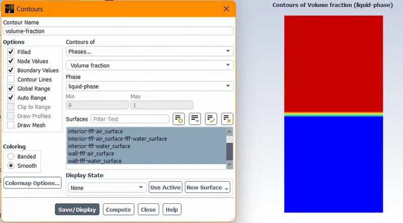
• Upper Portion represents Water(`α = 1`)
• Lower Portion Represents Air ( `α = 0` )
• Initiazilation Method -> Hybrid
• Solving Method -> PISO
• Total Flow Time = (Time Step Size) * (No of Time Steps)

Post-Processing Results

Case 1 Meshing The Geometry for BaseLine Mesh Simulation( i.e mesh size = 0.5 mm)

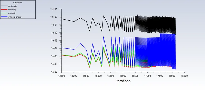
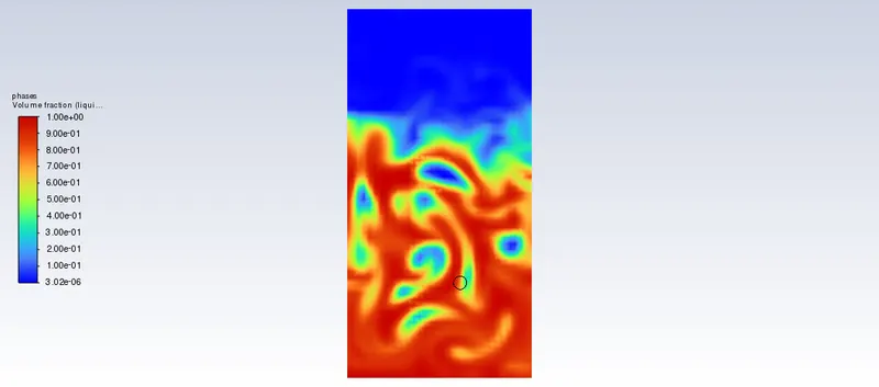
Video Animation Link

https://drive.google.com/file/d/1e9Rrnf2PrQgHwAyUZjaLSvdIDkuol7hA/view?usp=share_link

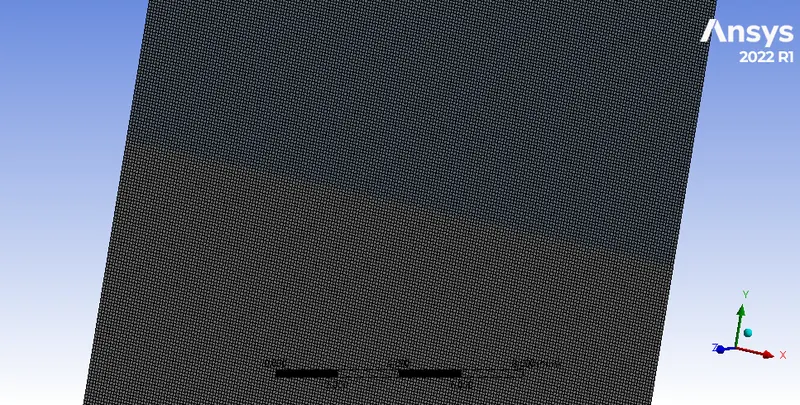
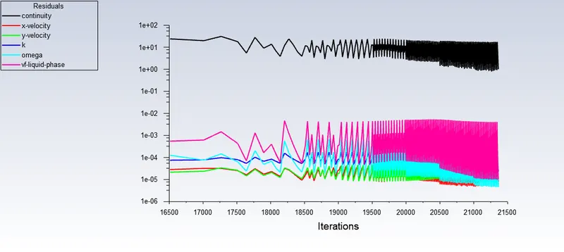
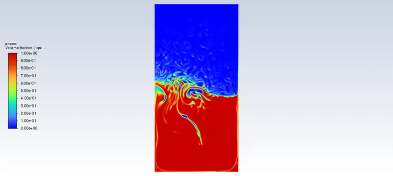
Case 2 Meshing The Geometry for Refined Mesh Simulation( i.e mesh size = 0.1 mm)

Video Animation Link

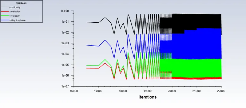
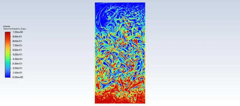
Case 3 Meshing The Geometry for Refined Mesh Simulation( i.e mesh size = 0.1 mm) with water and user-defined-material(density = 400 kg/m³, viscosity = 0.001 kg/m-s)

Video Animation Link

4. Define the Atwood Number. Find out the Atwood number for both the cases and explain how the variation in Atwood number in the above two cases affects the behavior of the instability.

• In fluid dynamics, the Atwood Number is described as a dimensionless number that is used to explore hydrodynamic instabilities in density-stratified flows.
• It is the ratio of difference in densities to the summation of the densities

`A = (ρ1 - ρ2)/(ρ1 + ρ2) `

where, A = Atwood number, ρ1 = density of fluid 1, ρ2 = density of fluid 2.

Calculation Results Table

Mesh Type	Mesh Size	Materials Used	Atwood Number
BaseLine Mesh Simulation	0.5 mm	Air and water-liquid	0.99754
Refined Mesh Simulation	0.1 mm	Air and water-liquid	0.99754
Refined Mesh Simulation	0.1 mm	user-defined-material and water-liquid	0.42784

Conclusions

• For Atwood Number close to zero, Rayleigh Taylor Instability takes up the form of symmetric fingers of fluid.
• For Atwood Number close to one, Rayleigh Taylor Instability the lighter fluid takes up the form of larger bubble-like plumes.
• As steady state approach is time independent and in our simulations we need to study the time dependent physics of turbulent mixing nature of two fluids which is frequently changing with respect to time.