Week 5 - Rayleigh Taylor Instability

Aim--> Demonstration of Rayleigh-Taylor Instabilities

Rayleigh-Taylor Instabilities

Named after Lord Rayleigh and G.I. Taylor

It is the instability of an interface between two fluids of different densities which occurs when the lighter fluid is pushing the heavier fluid. Examples are water suspended above the oil in gravity action, nuclear explosions, volcanic eruptions etc. Water suspended atop oil is an everyday example of Rayleigh–Taylor instability, and it may be modelled by two completely plane-parallel layers of immiscible fluid, the denser on top of the less dense one and both subject to the Earth's gravity. The equilibrium here is unstable to any perturbations or disturbances of the interface: if a parcel of heavier fluid is displaced downward with an equal volume of lighter fluid displaced upwards, the potential energy of the configuration is lower than the initial state. Thus, the disturbance will grow and lead to a further release of potential energy, as the denser material moves down under the (effective) gravitational field, and the less dense material is further displaced upwards. This was the set-up as studied by Lord Rayleigh. The important insight by G. I. Taylor was his realisation that this situation is equivalent to the situation when the fluids are accelerated, with the less dense fluid accelerating into the more dense fluid. This occurs deep underwater on the surface of an expanding bubble and in a nuclear explosion.

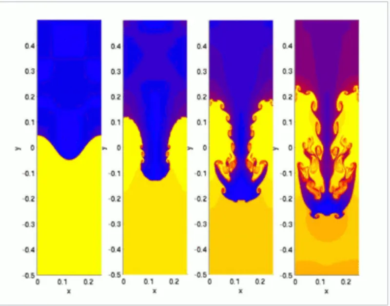
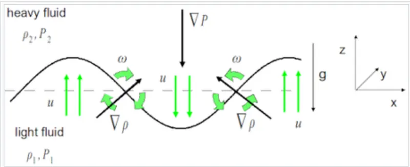
As the RT instability develops, the initial perturbations progress from a linear growth phase into a non-linear growth phase, eventually developing "plumes" flowing upwards (in the gravitational buoyancy sense) and "spikes" falling downwards. In the linear phase, the fluid movement can be closely approximated by linear equations, and the amplitude of perturbations is growing exponentially with time. In the non-linear phase, perturbation amplitude is too large for a linear approximation, and non-linear equations are required to describe fluid motions. In general, the density disparity between the fluids determines the structure of the subsequent non-linear RT instability flows (assuming other variables such as surface tension and viscosity are negligible here). The difference in the fluid densities divided by their sum is defined as the Atwood number, (A). For (A) close to 0, RT instability flows take the form of symmetric "fingers" of fluid; for (A) close to 1, the much lighter fluid "below" the heavier fluid takes the form of larger bubble-like plumes.

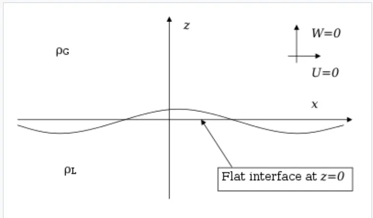
Stages of development and eventual evolution into turbulent mixing

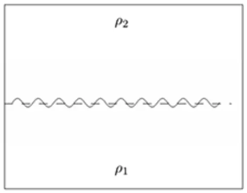
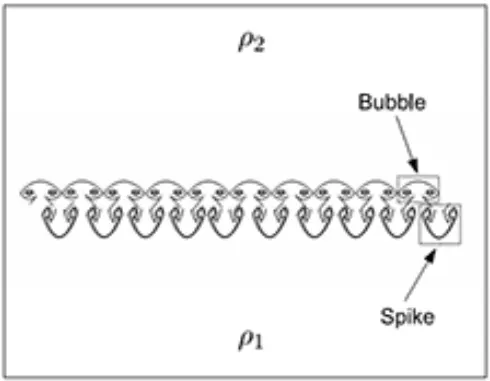
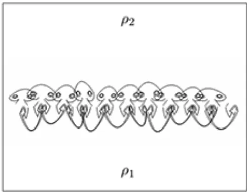
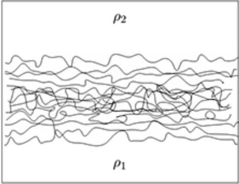
The evolution of the RTI follows four main stages. In the first stage, the perturbation amplitudes are small when compared to their wavelengths, the equations of motion can be linearized, resulting in exponential instability growth. In the early portion of this stage, a sinusoidal initial perturbation retains its sinusoidal shape. However, after the end of this first stage, when non-linear effects begin to appear, one observes the beginnings of the formation of the ubiquitous mushroom-shaped spikes (fluid structures of heavy fluid growing into light fluid) and bubbles (fluid structures of light fluid growing into heavy fluid). The growth of the mushroom structures continues in the second stage and can be modelled using buoyancy drag models, resulting in a growth rate that is approximately constant in time. At this point, nonlinear terms in the equations of motion can no longer be ignored. The spikes and bubbles then begin to interact with one another in the third stage. Bubble merging takes place, where the nonlinear interaction of mode coupling acts to combine smaller spikes and bubbles to produce larger ones. Also, bubble competition takes places, where spikes and bubbles of smaller wavelength that have become saturated are enveloped by larger ones that have not yet saturated. This eventually develops into a region of turbulent mixing, which is the fourth and final stage in evolution. It is generally assumed that the mixing region that finally develops is self-similar and turbulent, provided that the Reynolds number is sufficiently large.

Kelvin-Helmholtz instability

The Kelvin–Helmholtz instability (after Lord Kelvin and Hermann von Helmholtz) typically occurs when there is velocity shear in a single continuous fluid, or additionally where there is a velocity difference across the interface between two fluids. A common example is seen when the wind blows across a water surface; the instability constant manifests as waves. Kelvin-Helmholtz instabilities are also visible in the atmospheres of planets and moons, such as in cloud formations on Earth or the Red Spot on Jupiter.

The theory predicts the onset of instability and transition to turbulent flow within fluids of different densities moving at various speeds. Helmholtz studied the dynamics of two fluids of different densities when a small disturbance, such as a wave, was introduced at the boundary connecting the fluids. Kelvin–Helmholtz instability can thus be characterized as unstable small-scale motions occurring vertically and laterally

Richtmyer–Meshkov instability

The Richtmyer–Meshkov instability (RMI) occurs when two fluids of different density are impulsively accelerated. Normally this is by the passage of a shock wave. The development of the instability begins with small amplitude perturbations which initially grow linearly with time. This is followed by a nonlinear regime with bubbles appearing in the case of a light fluid penetrating a heavy fluid, and spikes appearing in the case of a heavy fluid penetrating a light fluid. A chaotic regime eventually is reached and the two fluids mix. This instability can be considered the impulsive-acceleration limit of the Rayleigh–Taylor instability.

Plateau–Rayleigh instability

The Plateau–Rayleigh instability, often just called the Rayleigh instability, explains why and how a falling stream of fluid breaks up into smaller packets with the same volume but less surface area. It is related to the Rayleigh–Taylor instability and is part of a greater branch of fluid dynamics concerned with fluid thread breakup. This fluid instability is exploited in the design of a particular type of inkjet technology whereby a jet of liquid is perturbed into a steady stream of droplets.

The driving force of the Plateau–Rayleigh instability is that liquids, by virtue of their surface tensions, tend to minimize their surface area. A considerable amount of work has been done recently on the final pinching profile by attacking it with self-similar solutions.

Geometry of the problem

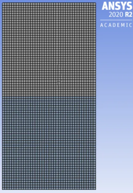
Following is the geometry of the problem, bottom part represents the lighter fluid and the top part represents the more dense fluid. At the interface mesh has to be shared by both the fluids i.e. mesh must be conformal. The boundaries represent the walls. Individual boxes are 20 mm in length and height.

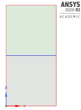
Air (bottom)

Water (Top)

Mesh

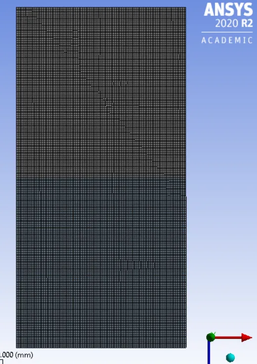
For the current case we use 2 meshes, Base-mesh and refined mesh. We observe the patterns for the rayleigh-taylor waves.

1. Base-mesh --> element size -- 0.5 mm

nodes -- 3321

elements -- 3200

2. Refined Mesh --> element size -- 0.2 mm

nodes -- 20301

elements -- 20000

Results

Case 1

1. Base-Mesh

--> We use transient simulation for this type of simulation. We are using Volume of Fluid method (VOF) in Ansys fluent solver.

Viscous model -- Laminar

Time-step -- 0.05 s

2. Refined-Mesh

Viscous model -- Laminar

Time-step -- 0.005 s

3. User-defined Material -->

density = 400 kg/m3

viscosity = 0.001 kg/m-s

Defination of Atwood Number

It is a non dimensional constant in fluid dynamics which is used in the study of hydrodynamical instabilities in density stratified flows. It is a dimensionless density ratio. It is given as follows -->

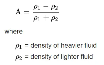
Atwood number is an important parameter in the study of Rayleigh–Taylor instability and Richtmyer–Meshkov instability. In Rayleigh–Taylor instability, the penetration distance of heavy fluid bubbles into the light fluid is a function of acceleration time scale Agt^2 where g is the gravitational acceleration and t is the time.

ρ1 = 997

ρ2 = 1.225

A = 0.99754

Thus, Atwood Number in our case is 0.99754.