Week 5 - Rayleigh Taylor Instability

AIM:-

• To run the Simulation for Rayleigh-Taylor-Instability Using Ansys-Fluent.

OBJECTIVES:-

• What are the Some CFD models that have been based on the mathematical analysis of Rayleigh-Taylor-Instability Waves.
• To Perform the Rayleigh-Taylor-Instability Simulation for 2 different Mesh Size with the Base Mesh being 0.5mm.
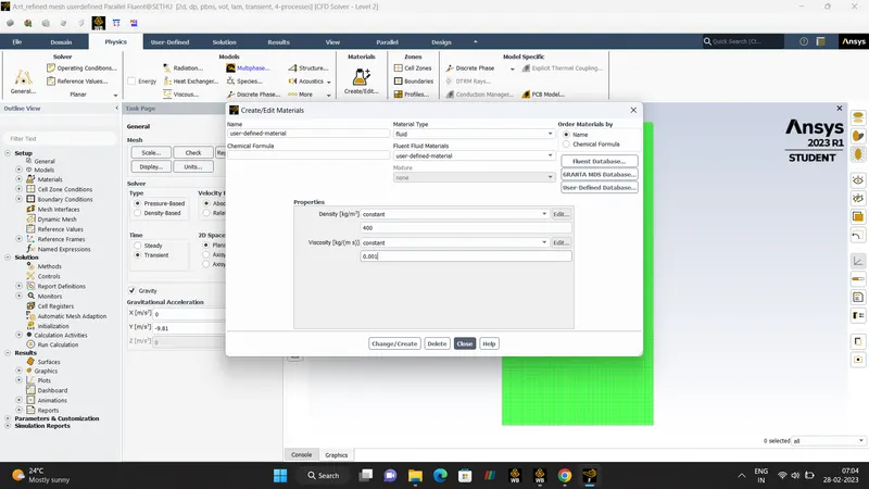
• To run the Simulation with WATER and USER-DEFINED Material (Density - 400kg/m^3, Viscosity-0.001kg/m^-3) for Refined Mesh.
• Define ATWOOD NUMBER, Explain the Varaition of the atwood number affects the behaviour of instability.

PROCEDURE:-

Source (WIKIPEDIA)

DEFINITION - RAYLEIGH-TAYLOR-INSTABILITY.

• Introduced by LORD RAYLEIGH and G.I TAYLOR.
• Rayleigh-Taylor-Instability or RT-Instability is the interpenetration of materials that occurs whenever a light fluid pushes on a heavy fluid.
• It is a Dynamic process whereby the two fluids seek to reduce their combined potential energy.
• The ensuring turbulence and mixing has far-reaching consequences in many natural and man-made flours,ranging from supernova to inertial confinement fusion(ICF) capsules.

RAYLEIGH-TAYLOR-INSTABILITY.

• ABSTRACT.

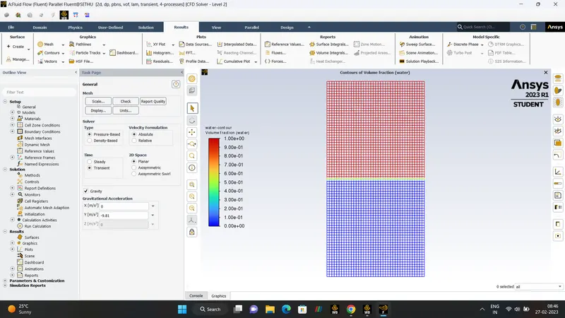
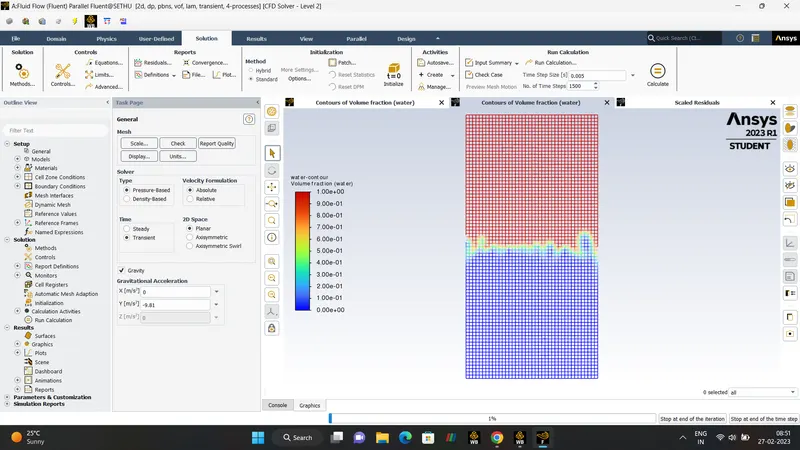
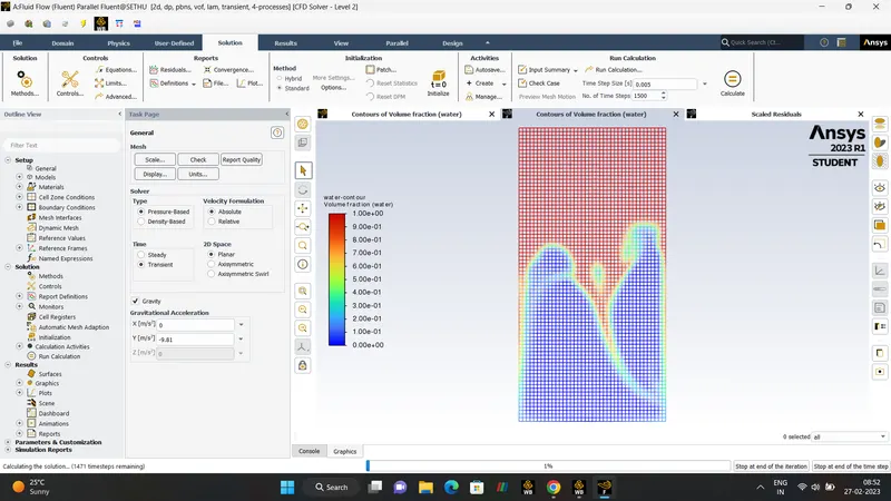
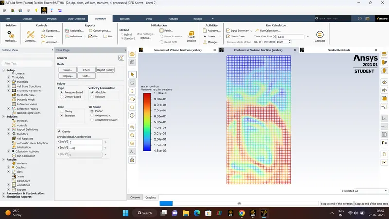
This Project is about Simulation of Rayleigh-Taylor-Instability of two fluids WATER and AIR. The fluid(WATER) with higher density is placed on the top region of the Surface and the fluid(AIR) with lesser density is placed in the bottom region of the Surface. This project is solved with ANSYS-FLUENT with k-EPSILON model with TRANSIENT-STATE simulation being used. In the third case setup file USER-MATERIAL is being used with (Density - 400kg/m^3, Viscosity-0.001kg/m^-3) for Refined Mesh.

• INTRODUCTION.

Rayleigh-Taylor-Instability or RT-Instability is the interpenetration of materials that occurs whenever a light fluid pushes on a heavy fluid. It is a Dynamic process whereby the two fluids seek to reduce their combined potential energy. The ensuring turbulence and mixing has far-reaching consequences in many natural and man-made flours,ranging from supernova to inertial confinement fusion(ICF) capsules.

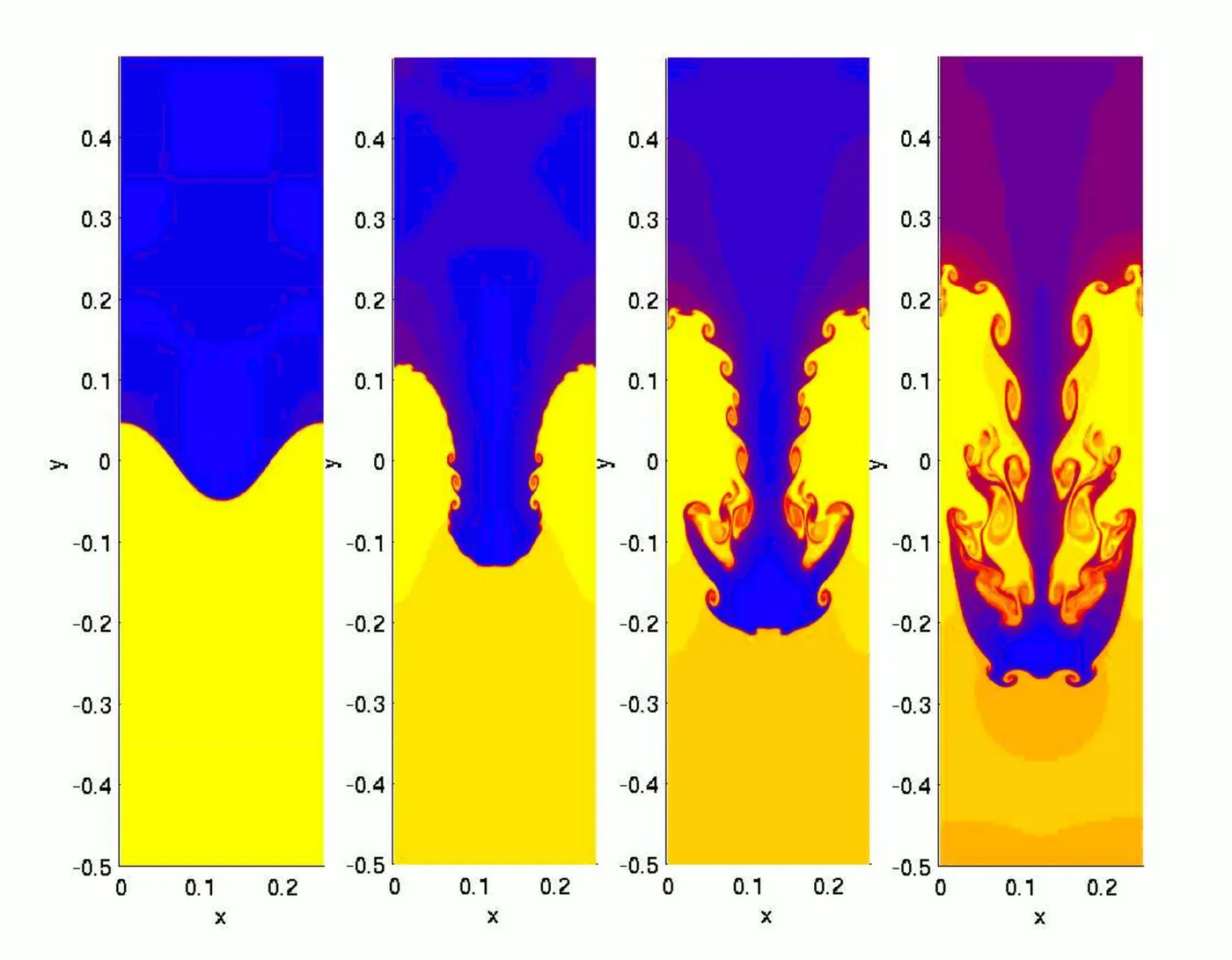
Water suspended a top oil is an everyday example of Rayleigh-Taylor-Instability and it may be modeled by two completely plane-parallel layers of immiscible fluid, the denser fluid on top of less dense one and both subject to the earth gravity. The equilibrium here is unstable to any perturbation or disturbance of the interface. If a parcel of heavier fluid is displaced downward with an equal volume of lighter fluid displaced upwards the potential energy of the configuration is lower than the initial state. Thus the disturbance will grow and lead to further release of the potential energy, as the denser material moves down the (effective) gravitational fluid,and the less dense material is further displaced upwards. This was the setup as studied by Lord Rayleigh. The important insight by G.I.Taylor was his realisation that this situation is equivalent to the simulation when the fluids are accelerated, with less dense fluid accelerating into dense fluid.This occurs deep underwater on the surface of an expanding buuble and in a nuclear explosion.

As the RT-Instability develops, the initial perturbation, from a linear growth phase into a non-linear growth phase, eventually developing 'Plumes' flowing upwards( in gravitational buoyancy sense) and spikes falling downwards. In this LINEAR PHASE, the equation can be linearized and the amplitude of the perturbation is growing exponentially with time.

In the NON-LINEAR PHASE, perturbation amplitude is too large for the non-linear term to be neglected. In ground the density disparity between the fluids determine the structure of subsequent non-linear RT-Instability flow( assuming other variables such as Surface Tension and Viscosity are neglibile here).

• STAGES OF DEVELOPEMENT AND EVOLUTION INTO TURBULENT MIXING.

The Rayleigh-Taylor-Instability consists of four major stages.

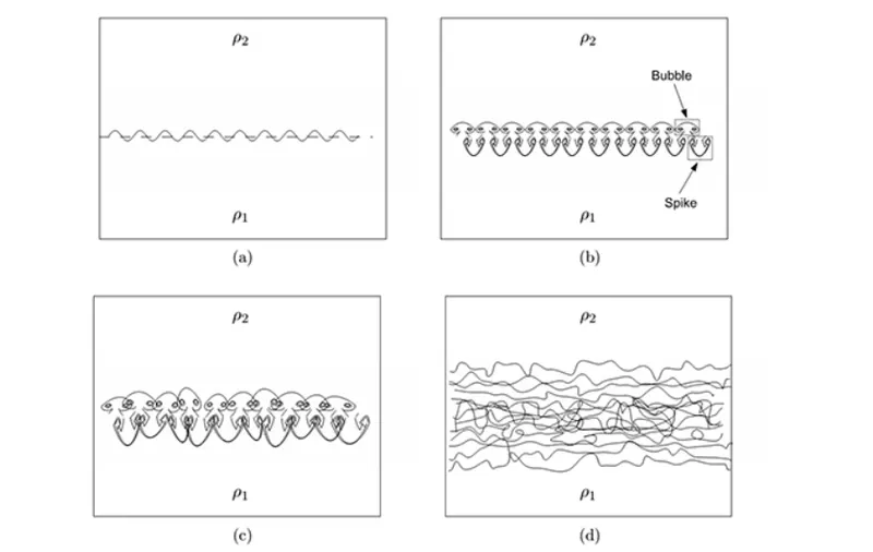
STAGE 1 - In this stage the perturbation amplitudes are small when compared to their wavelengths, the equation of motion can be linearized, resulting in exponential instability growth. In this stage, sinusoidal initial perturbation retains it's sinusoidal shape.

STAGE 2 - In this stage Non-Linear effects begin to appear, One observe the beginings of the formation of the ubiquitous mushroom. Shaped Spikes(fluid structures of heavy fluid growing into the light fluid) and the bubbles(fluid structures of light fluid growing into the heavy fluid). The growth of the mushroom structures continous in the second stage.

STAGE 3 - In this stage the Spikes and Bubbles begin to interact with one another, bubble merging takes place where the non-linear interactionof mode couplingacts to combine smaller spikes and bubbles produce larger ones. Also, bubble competition take places, where spikes and bubbles of smaller wavelength that have become saturated are envoloped by larger ones that have not yet saturated.

STAGE 4 - Turbulence mixing is happening in final stage of evolution. It is generally assumed that the mixing region that finally develops is semi-similar and turbulent, provided that Reynold's number is sufficiently large.

• PARTICLE CFD MODEL ON RAYLEGH TAYLOR INSTABILITY WAVES.

1. KELVIN-HELMHOLTZ-INSTABILIITY.

2. PLATEAU-RAYLEIGH-INSTABILITY.

KELVIN-HELMHOLTZ-INSTABILITY.

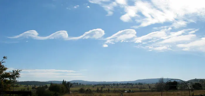
This stability occurs when there is a velocity shear in a single continous or there is velocity difference across the interference between the two fluids. For example when a wind flows across a water surfaces. The instability constant is able to manifest itself through waves on a water surfaces. The kelvin-helmholtz instability is not only restricted to the water surface as clouds, but it evidence through the other natural phenomena as Ocean and sun corona's. The theory predicts the onset of instability and transition to turbulent flow in fluids of different densities moving at various speeds. This Instabilities occurs where there is a velocity shear or velocity difference between the interference of the two fluids.

PLATEAU-RAYLEIGH-INSTABILITY.

Plateau-rayleigh-Instability, often called as Rayleigh-Taylor-Instability, explains why and how a falling stream of fluids breaks up into smaller packests with the same volume but less surface area. It is related to the rayleigh-taylor, and is part of greater branch of fluid dynamics concerned with fluid thread breakup. This fluid instability is exploitted in design of a particular type of ink-jet technology whereby a jet of liquid is perturbed into a steady-stream of objects.

The driving force of the Plateau–Rayleigh instability is that liquids, by virtue of their surface tension, tend to minimize their surface area. A considerable amount of work has been done recently on the final pinching profile by attacking it with self similar solutions.

KEYWORDS :- MultiPhase, Volume Of Fluids, Transient-State.

MULTI-PHASE

MULTI-PHASE MODELLING.

DEFINITION:-

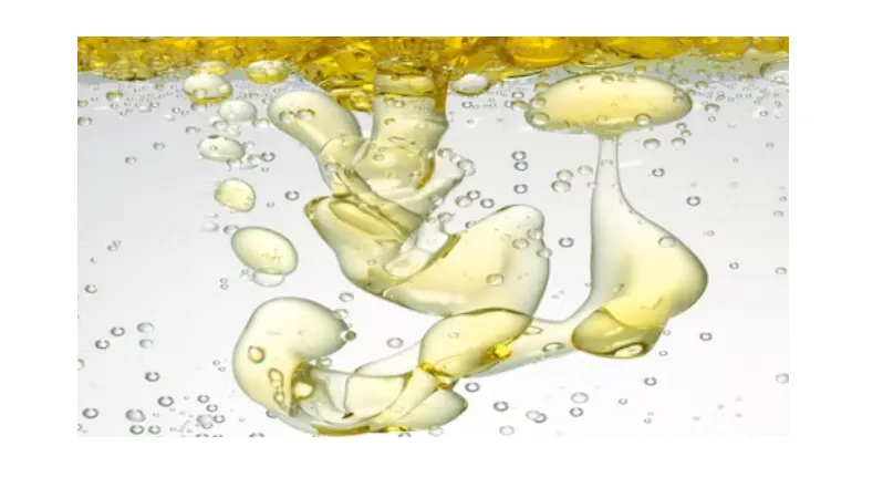
• Multiphase modelling is type of numerical analysis that deals with the modeling of two or more pahses of water interacting with one another in domain.
• For eg, oil despered in water. The two immiscible fluids, so the interaction of oil with the water can be tracked numerically as there will be an interface region betwee the two.

• SOLUTION FOR MULTIPHASE PROBLEM.

The most commonly used model in fluent are as follows,

1. Volume Of Fluid.

2. Mixture Model.

3. Eulerian Model.

4. Wet Stream Model.

• In this project, Volume of Fluid is used.

VOLUME OF FLUID.

DEFINITION:-

• Volume Of Fluid method is a surface tracking method. It is designed to find out the position of interface between the two-more immisicble fluids.
• The volume of fraction of each fluid in each of cell through out the domain can be tracked by using this methodand then in this method the single set of momentum equation is only shared by the fluids.
• In this method all control volumes must be filled with single phase of combination of phases.
• This method is only applicable for PRESSURE-BASED-SOLVERS.

TRANSIENT-STATE.

DEFINITION:-

• Transient Simulation computes the instantaneous values in each time for each quantity.
• Transient Simulation has much higher requirement compared to Steady-State.
• The Computational time is more less. The disk-Storage, evaluating results. Results of transient simulation may be more comprehensive than the Steady-State.

• CASE 1:-

MODEL - RAYLEIGH_TAYLOR_INSTABILITY.

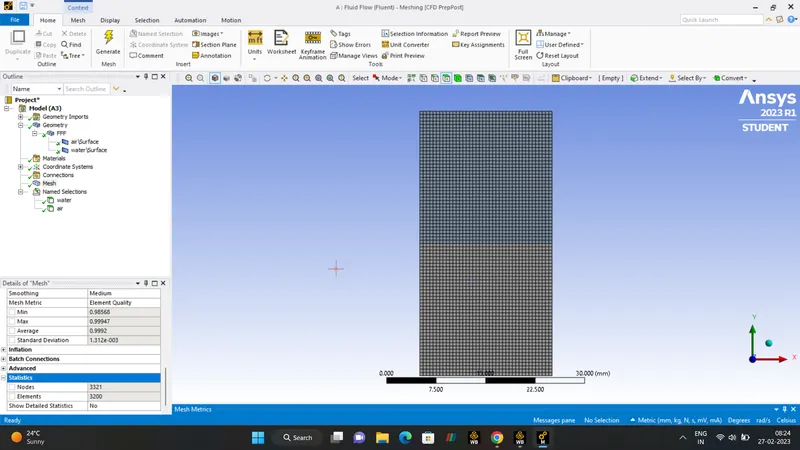
BASE LINE MESH 0.5 mm

GEOMETRY.

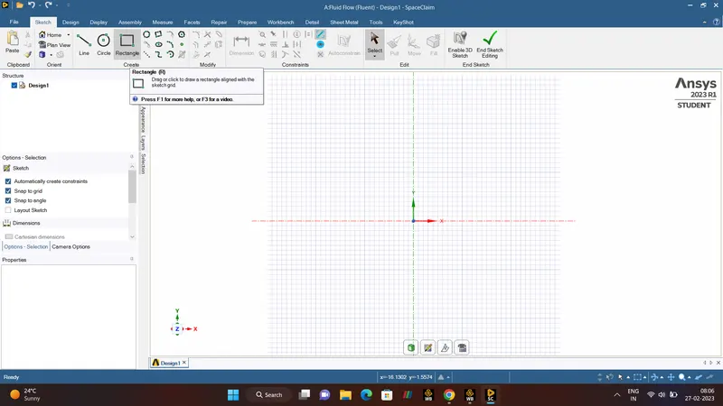
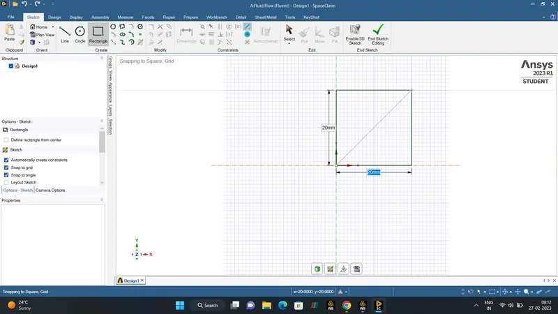
• In this project, let us dicuss about the 2D Simulation of Rayleigh-Taylor-Instability by using ANSYS-FLUENT. Open SpaceClaim create two squares 20mm*20mm with the rectangle tool.

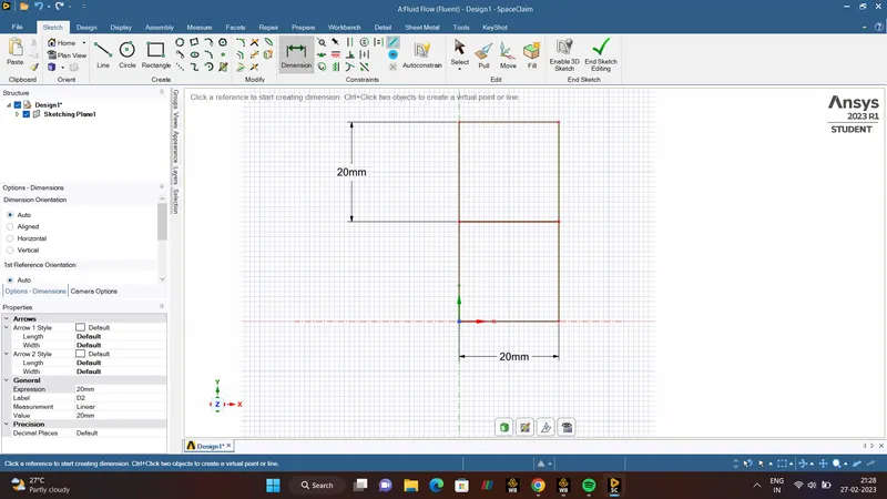
• After creating 2D geometry, with the help of pull tool two surfaces are made followed by AIR and WATER.

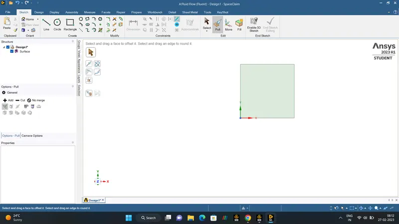
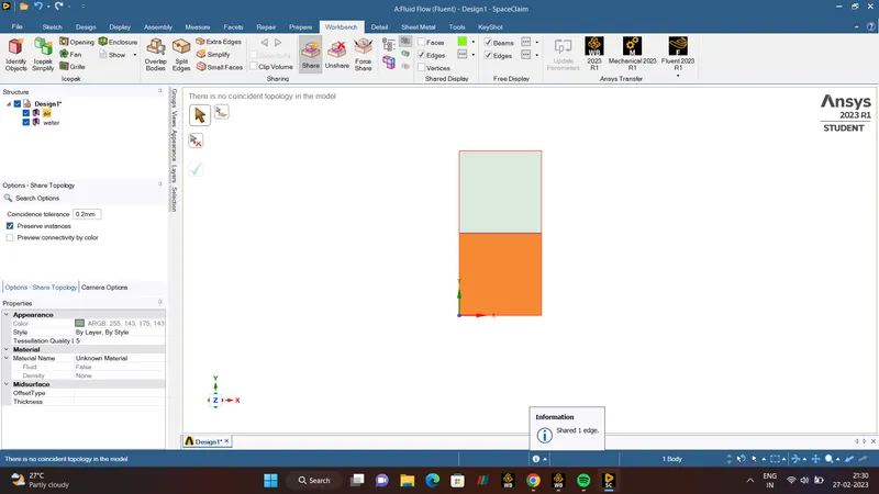
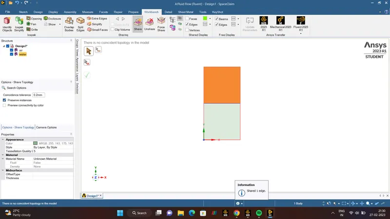
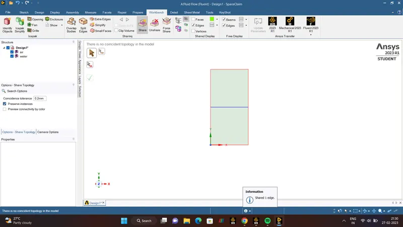
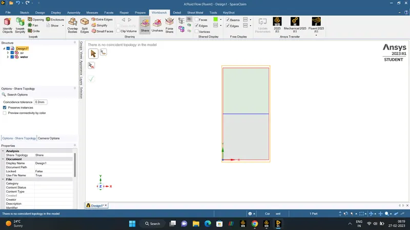
• Finally Share topology is to ensure that connected bodies have shared faces, which helps facilitate the creation of conformal mesh.

MESHING.

• Meshing, also known as the mesh operation which is process of generating the two or three dimesnional grids. It is dividing complex geometry into elements that can be used to discrete a domain.

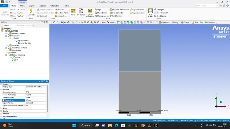
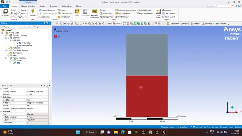
NAME SELECTION.

1. Water

2. Air

With the help of face selection tool (cntrl+F) the names are given.

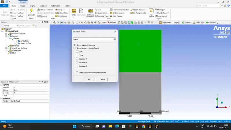
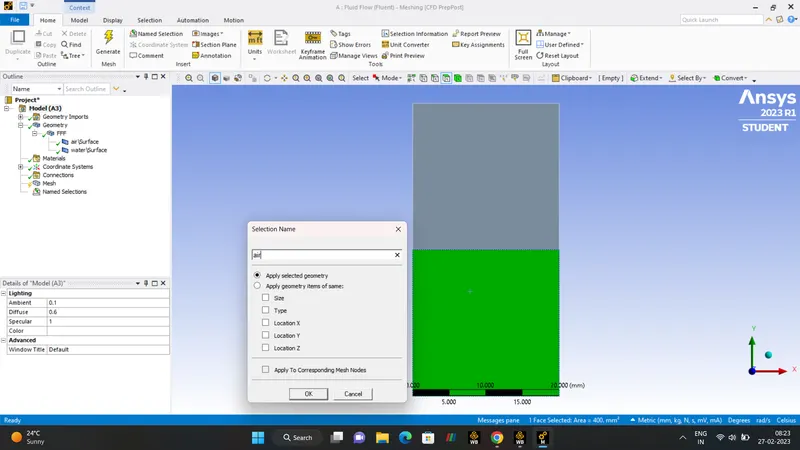
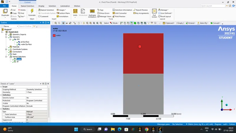
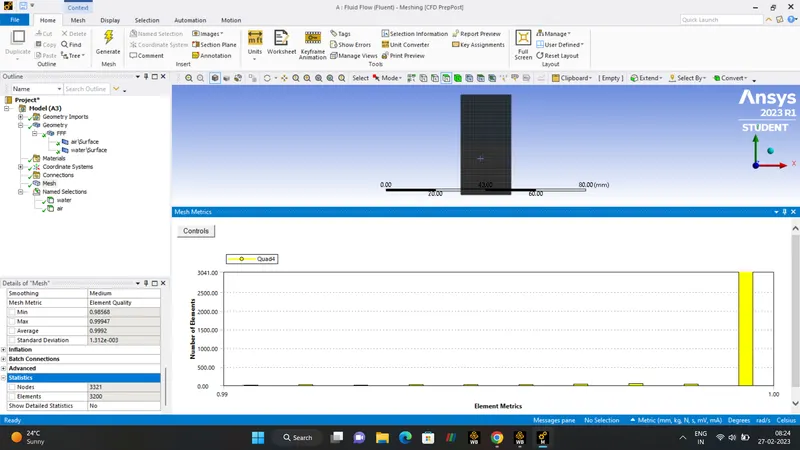
ELEMNET QUALITY.

SETUP.

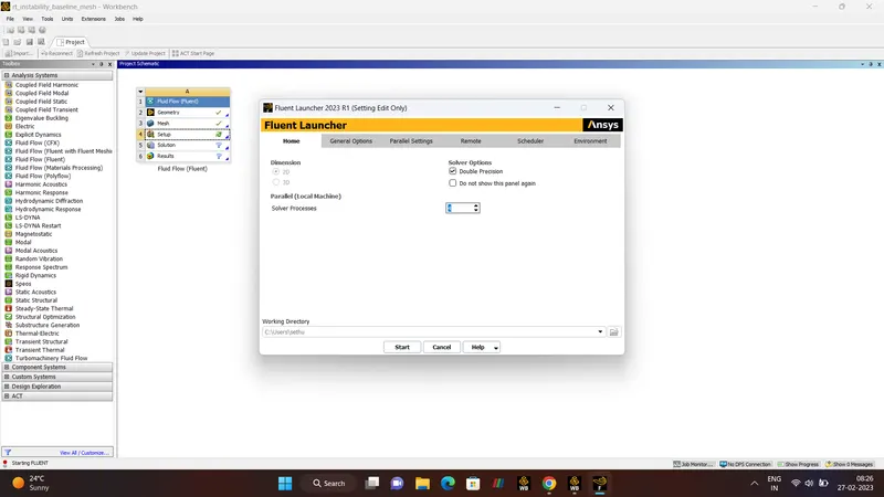
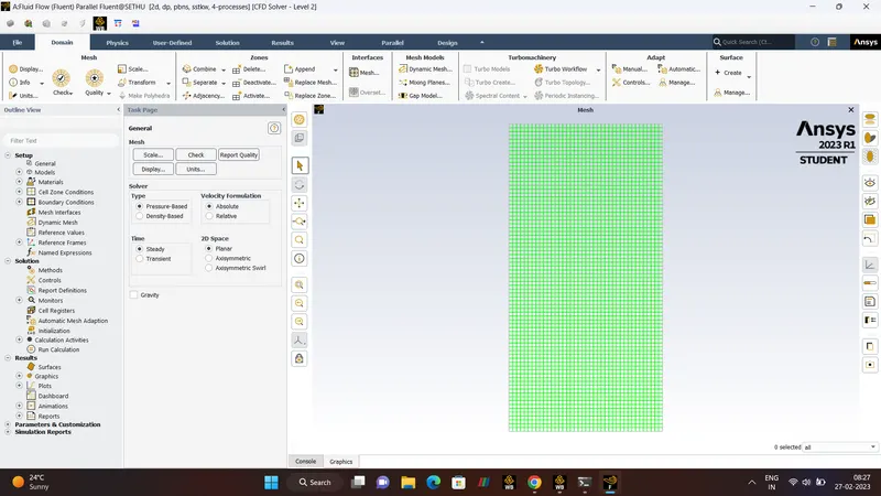
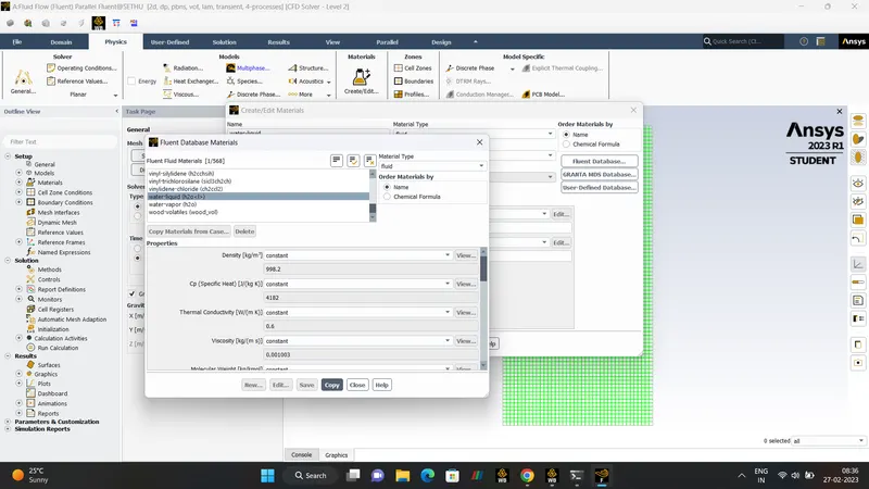
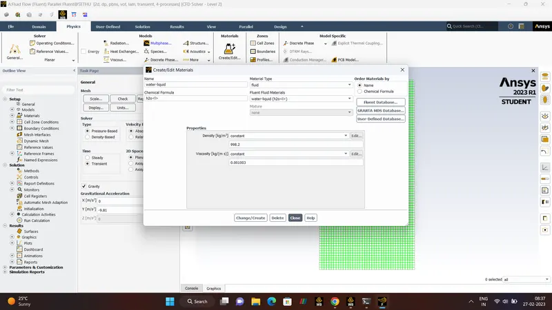
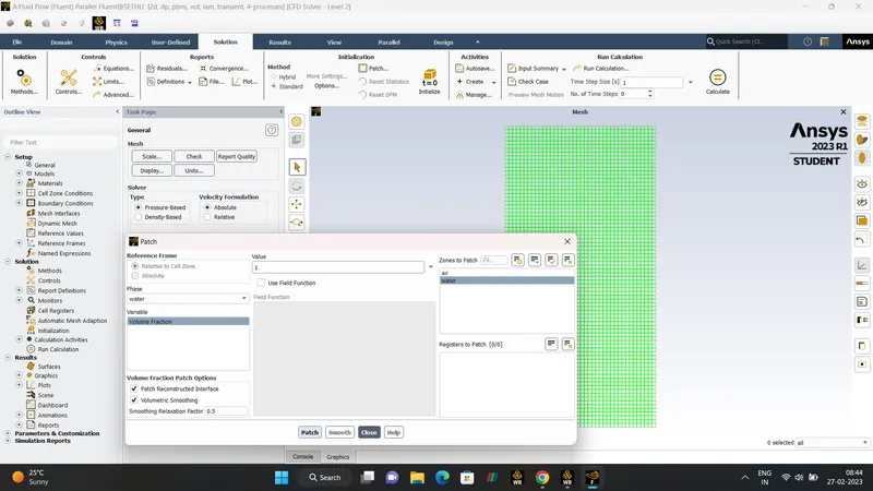
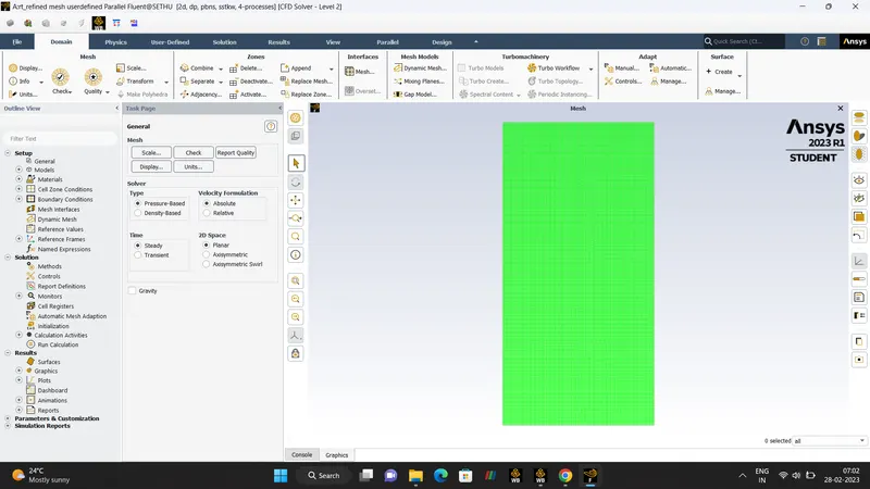
After creating the geometry and meshing is done, next step is to setting up the solution. Fluent Launcher `rarr` Double Precision `rarr`4 core. Check mesh is done.

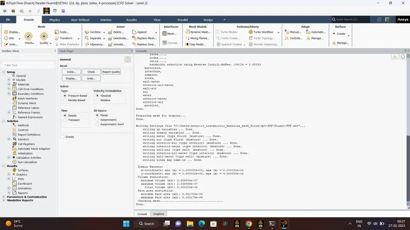
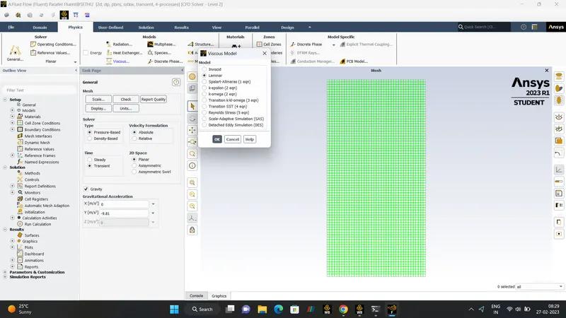
SOLVER	PRESSURE-BASED
TIME (STATE)	TRANSIENT-STATE
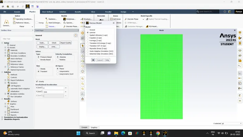
VISCOUS MODEL	LAMINAR
GRAVITY	-9.81 (y-axis)
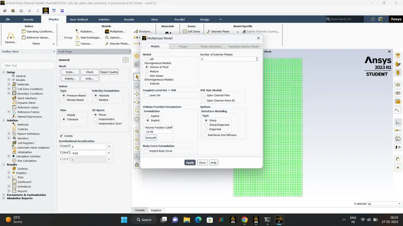
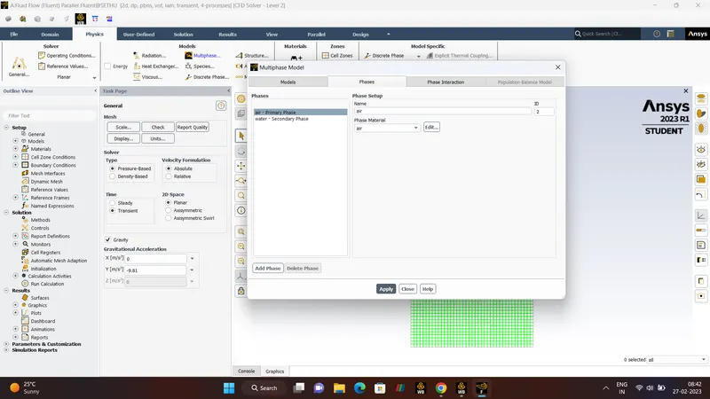
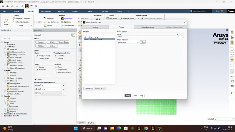
MULTIPHASE	VOLUME OF FLUIDS
FLUIDS	TWO (WATER-HEAVIER & AIR-LIGHT)
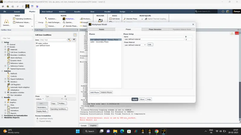
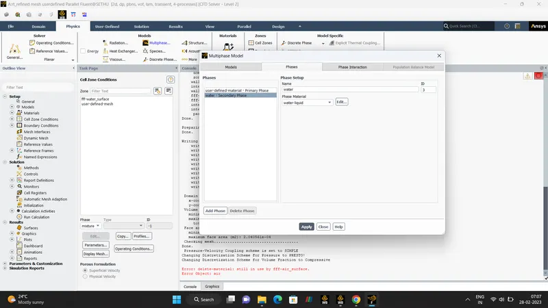
PHASES	PRIMARY-AIR & SECONDARY-WATER
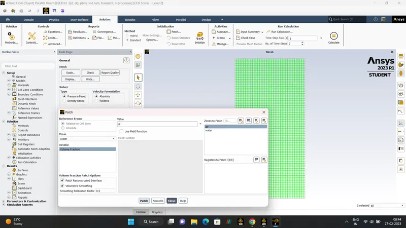
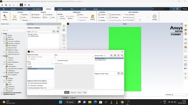
PATCH -Water(Voume Fraction)	WATER-1 & AIR-0
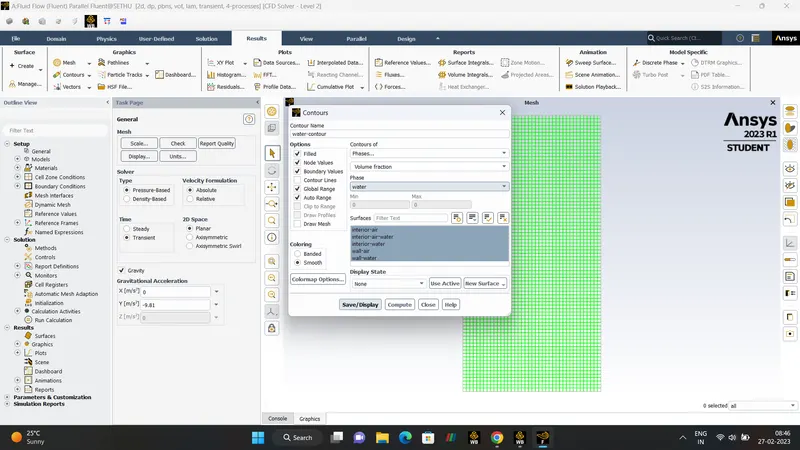
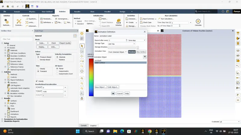
ANIMATION	WATER

RESULTS.

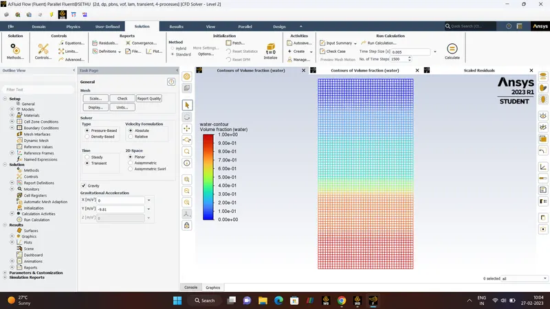
RESIDUALS.

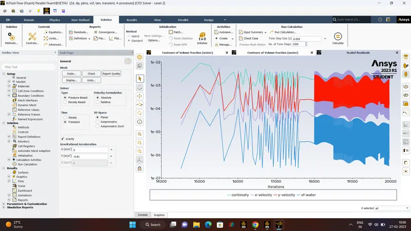
ANIMATION.

• CASE 2 -

Mesh size - 0.15mm

Surfaces - Water and Air.

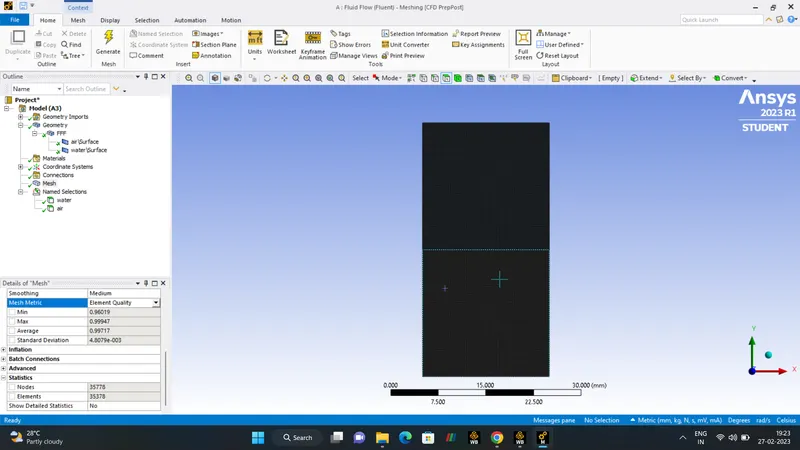
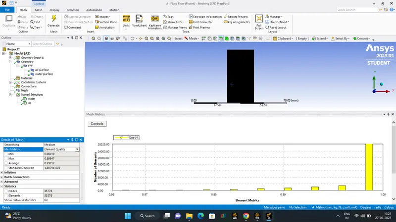
SETUP.

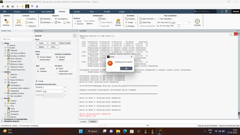
FLOATING-POINT-EXCEPTION.

DEFINITION:-

• Floating Point Exception means that the solvers detects an arithmetic Operation, which it cannot compute. For exmaple diversion of zero (or) if the number exceeds the bounds for the numerical data, types used in codes. Mathematically speaking we are dealing with the Divergence here.

How to Over-come the Floating Point Exception?.

1. Use Upwind Convection Scheme.

• Upwind convection scheme introduce numerical diffusion but ensure convergence in car train case. For Steady State simulation,'the bounded gauss upwind' schemes are more approach since they ensure boundedness. Try not to avoid higher-order scheme since they are more susceptile to divergence.

2. Double Check the Intial and Boundary Condition.

• Sometimes inital and boundary conditions led to Partial Difference Equation, check that we are not using zero for any,
• TURBULENT-KINETIC-ENERGY.
• TEMPERATURE.
• PRESSURE in a compressible flow.

note that zero Pressure is absolutely fine in In-compressible flow no equation of state is solved.

3. Limit The Time Step.

• Many Simulation types(most notably multiphase simulation using VOF method) are susceptible to a large time step.
• Especially during the first iterations, the flow velocities are Often still low and CFL criterion will cause the time step to choosing two big.

4. Solvers.

• Use COUPLED Solvers if possible.
• Choose GAMG and SMOOTH Solvers. Especially smooth Solvers performs quite well when the materials have bad conditions.

In Our Project, We Choose COUPLED SOLVERS.

5. Processor.

• Running in Series or Parallel with single processor sometimes help.

6. Mesh Quality.

• Check all Mesh Qualilty parameters and maintain the (Skewness under 0.8) aspect ratio within the approrate range. The Bad Mesh can lead to FLOATIING POINT EXCEPTION ERROR. Try to use conformal mesh because interface can prone to give this error.

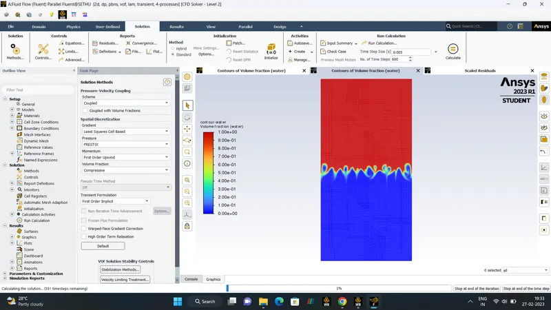
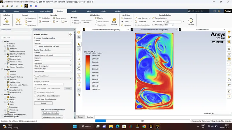
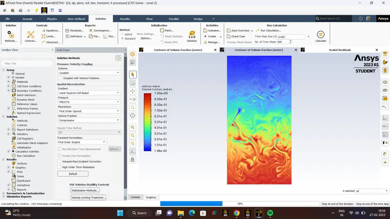
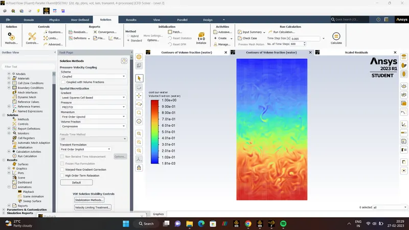
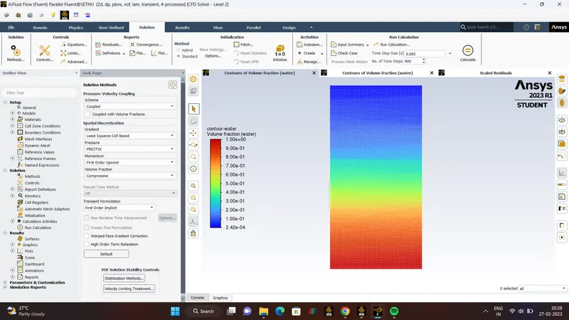
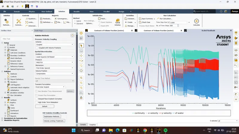
In Our Project, First We Choose More REFINED MESH, Mesh Element around 0.1mm, the solution cameup with the Floating Point Error which leads to DIVERGENCE, So again we changed the MESH from 0.1mm to 0.18mm`rarr`COUPLED SOLVERS `rarr`FIRST ORDER UPWIND`rarr`Reduced TIME STEP from 700 to 600 Solution`rarr` CONVERGENCE.

RESULTS.

RESIDUALS.

ANIMATION.

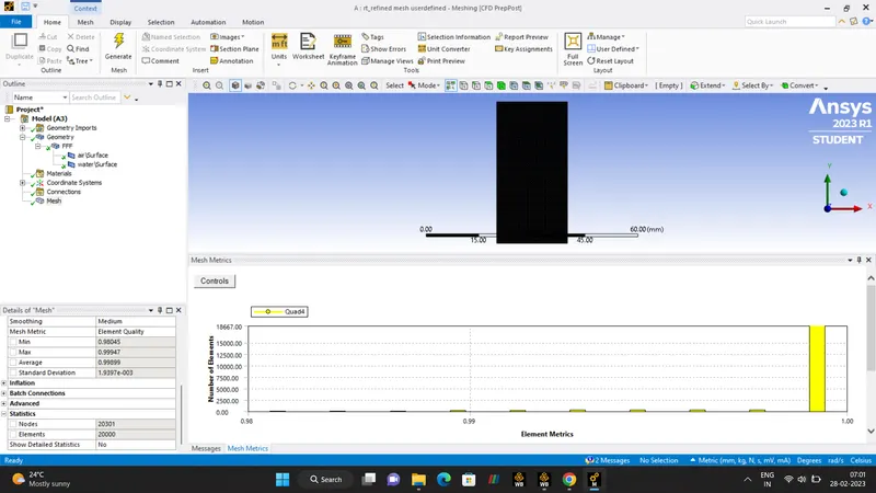
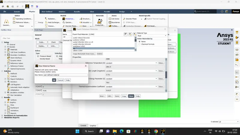
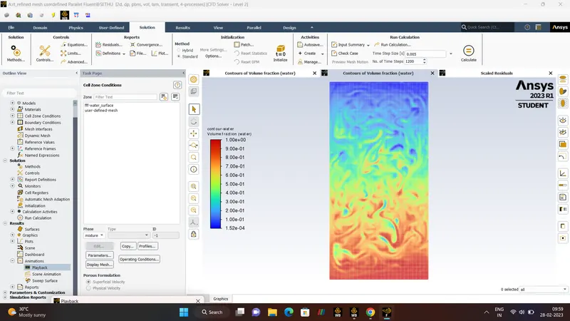
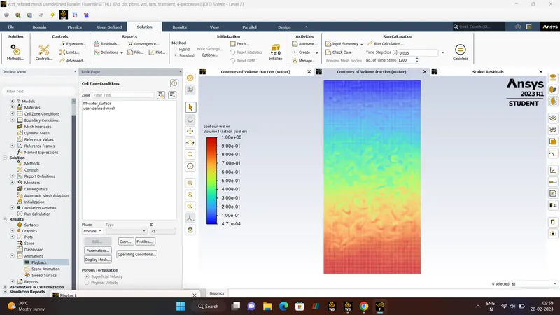
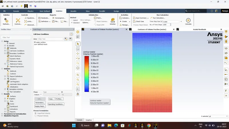
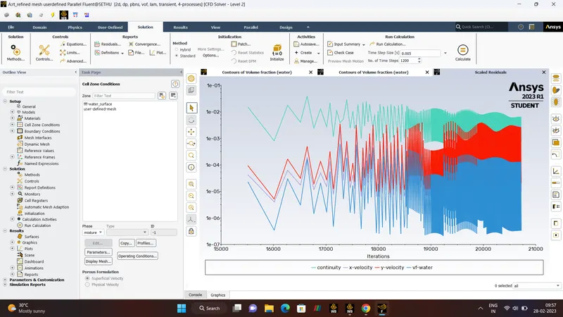
• CASE 3-

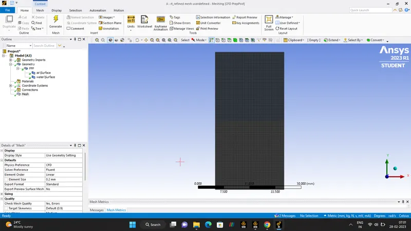
Mesh Size - 0.2mm

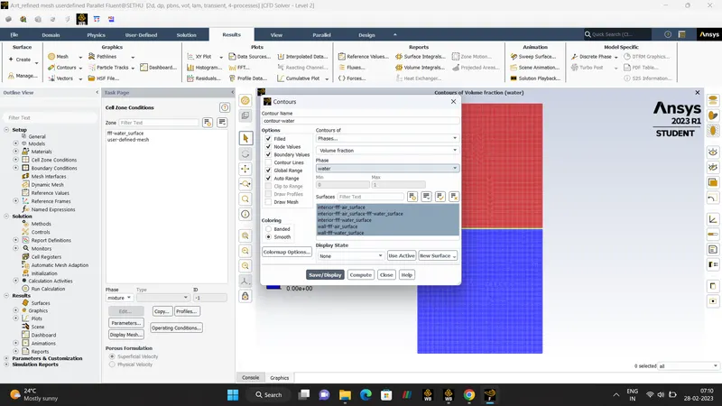
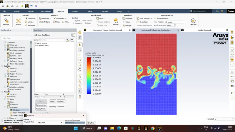
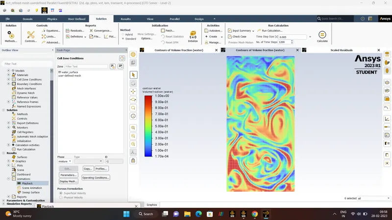
Surfaces - Water and User-Defined-Material (Density 400 kg/m^3 and Viscosity 0.001 kg/m-s).

RESIDUALS.

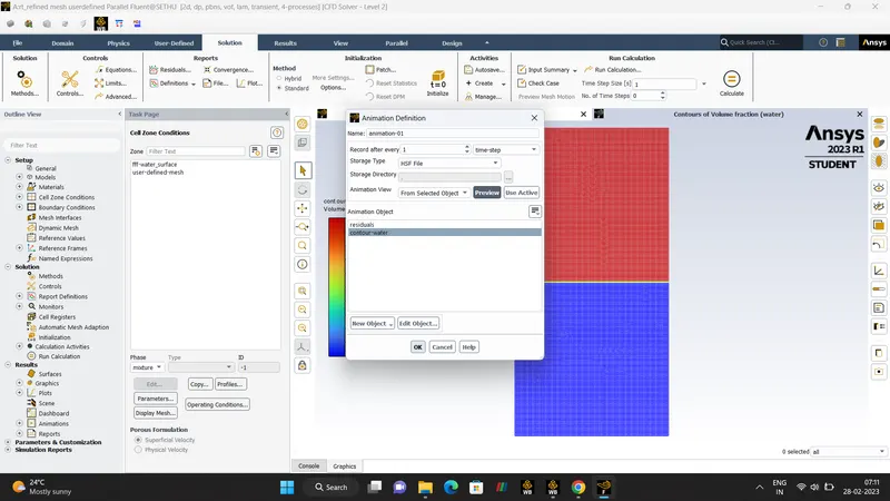
ANIMATION.

ATWOOD NUMBER.

DEFINITION:-

• Atwood Number is a dimensionless number in fluid dynamics used in the study of hyrodynamics instabilities in density strafified flows. It is a dimensionless ratio defined as

`A = (rho_1-rho_2)/(rho_1+rho_2)`

`rho_1 - Density of heavier fluids`

`rho_2 - Density of light fluids`

Case 1.

`rho_1 rarr water rarr heavier fluid rarr 998.2 (kg)/m^3`

`rho_2 rarr air rarr lighter fluid rarr 1.225 (kg)/m^3`

`A = (rho_1-rho_2)/(rho_1+rho_2)`

`A = (998.2-1.225)/(998.2+1.225)`

`A = 996.975/999.425 rarr 0.998`

Case2.

`rho_1 rarr water rarr heavier fluid rarr 998.2 (kg)/m^3`

`rho_2 rarr user-material rarr light fluid rarr 400 (kg)/m^3`

`A = (rho_1-rho_2)/(rho_1+rho_2)`

`A = (998.2-400)/(998.2+400)`

`A = 598.2/1398.2 rarr 0.427`

NO	FLUIDS	ELEMENT SIZE	NUMBER OF ELEMENTS	NUMBER OF TIME STEPS	ATWOOD NUMBER
1	WATER & AIR	0.5mm	3200	1500	0.998
2	WATER & AIR	0.15mm	35378	600	0.998
3	WATER & USER_DEFINED_MATERIAL	0.2mm	20000	1200	0.427

Why Steady-State Approach is not Siutable for this simulation?

• Steady-State approach is Time-Independent.
• Therefore, it never shows the flow changes with respect to time.
• The flow changes can be captured only in the transient-state.

CONCULSION:-

• Let us conclude from the above project, The Rayleigh-Taylor-Instability simulation for different mesh element is done, with following the base mesh.
• With more Refined mesh, Rayleigh Taylor Instability shows the better compared to the base mesh 0.5mm.
• With more Refined mesh, the computational time takes more time, compared to the baseline mesh.
• In this project, Transient-State Simulation is choosen over the Steady-State because Steady-state simulates the problem using iterative techinque.
• In this project, with more REFINED MESH of 0.1mm'FLOATING POINT EXCEPTION ERROR' occurs to overcome the error, few changes made, following the solution been Converged.