Rayleigh Taylor Instability

Aim :

• Perform the Rayleigh Taylor instability simulation for 2 different mesh sizes and also by using user defined fluid in another case with refine mesh and compare the results.

Objectives:

1. What are some practical CFD models that have been based on the mathematical analysis of Rayleigh Taylor waves? In your own words, explain how these mathematical models have been adapted for CFD calculations.
2. Perform the Rayleigh Taylor instability simulation for 2 different mesh sizes with the base mesh being 0.5 mm. Compare the results by showing the animations( Attach them from your Google drive). Observe the differences in the animation and explain the effect of mesh size on simulation. Also, explain why a steady-state approach might not be suitable for these types of simulation.[ Choose Air and Water for this simulation]
3. Run one more simulation with water and user-defined material(density = 400 kg/m3, viscosity = 0.001 kg/m-s) for refined mesh.
4. Define the Atwood Number. Find out the Atwood number for both the cases and explain how the variation in Atwood numbers in the above two cases affects the behaviour of the instability.

Theory :

1. Rayleigh-Taylor Instability (RT instability):

• Rayleigh- Taylor instability is the interpenetration of materials that occurs whenever the light fluid pushes on a heavy fluid.
• It is a dynamic process whereby the two fluids seek to reduce their combined potential energy.
• The ensuing turbulence and mixing has far reaching consequences in many natural and man-made flows, ranging from supernovae to initial confinement fusion (ICF) capsules.
• Ex:

1. The behaviour of water suspended above oil due to gravity effect of earth
2. Mushroom clouds like those from volcanic eruptions
3. Atmospheric nuclear explosions etc.

2. Some practical CFD models that have been based on the mathematical analysis of Rayleigh Taylor waves :

2.1. Mashroom clouds :

• A mushroom cloud is a distinctive mushroom-shaped flammagenitus cloud of debris, smoke and usually condensed water vapor resulting from a large explosion. The effect is most commonly associated with a nuclear explosion, but any sufficiently energetic detonation or deflagration will produce the same effect. They can be caused by powerful conventional weapons, like thermobaric weapons, including the ATBIP and GBU-43/B Massive Ordnance Air Blast. Some volcanic eruptions and impact events can produce natural mushroom clouds.

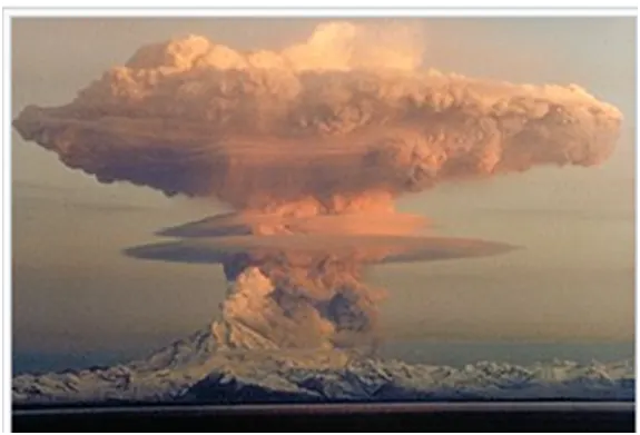
Fig : Mushroom cloud from Redoubt Volcano

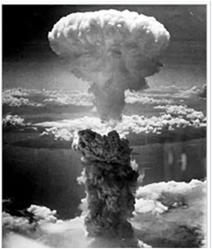
Fig : Mushroom cloud from the atomic bombing of Nagasaki, Japan

2.2. Plateau-Rayleigh instability :

• The Plateau–Rayleigh instability, often just called the Rayleigh instability, explains why and how a falling stream of fluid breaks up into smaller packets with the same volume but less surface area. It is related to the Rayleigh–Taylor instabilityand is part of a greater branch of fluid dynamics concerned with fluid thread breakup. This fluid instability is exploited in the design of a particular type of ink jet technology whereby a jet of liquid is perturbed into a steady stream of droplets.
• The driving force of the Plateau–Rayleigh instability is that liquids, by virtue of their surface tensions, tend to minimize their surface area. A considerable amount of work has been done recently on the final pinching profile by attacking it with self-similar
• Ex :

i) Water droping from a tap

ii) Urination

iii) Inkjet printing

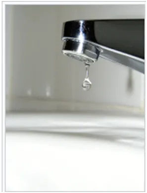
Fig : water dropping from tap

2.3. Richtmyer-Meshkov Innstability(RMI) :

• The Richtmyer–Meshkov instability (RMI)occurs when two fluids of different density are impulsively accelerated. Normally this is by the passage of a shock wave. The development of the instability begins with small amplitude perturbations which initially grow linearly with time. This is followed by a nonlinear regime with bubbles appearing in the case of a light fluid penetrating a heavy fluid, and with spikes appearing in the case of a heavy fluid penetrating a light fluid. A chaotic regime eventually is reached and the two fluids mix. This instability can be considered the impulsive-acceleration limit of the Rayleigh–Taylor instability.
• Ex : During the implosion of an inertial confinement fusion target, the hot shell material surrounding the cold D-T fuel layer is shock-accelerated. This instability is also seen in Magnetized target fusion. Mixing of the shell material and fuel is not desired and efforts are made to minimize any tiny imperfections or irregularities which will be magnified by RMI.

3. Multiphase :

• Multiphase flow is a simultaneous(parallel) flow of materials with different states or phases.(Ex: Liquid-Gas)
• It is a flow of materials with different chemical properties but in the same state or phase.(Ex: Liquid-Liquid or Gas-Gas)

3.1. Types of phases in multiphase :

• There are 3 types of phases in multiphase

1. Separated phase: Separated phase is defined as the one or more immiscible fluids in a continuous phase separated by an interface.
2. Dispersed Phase : It is defined as the phase in which the finite number of phases are spread in the continuous phase.
3. Mixed phase/Transient phase : It is defined as the phase in which one or more fluids mixed together. It contains both the separate and dispersed phases.

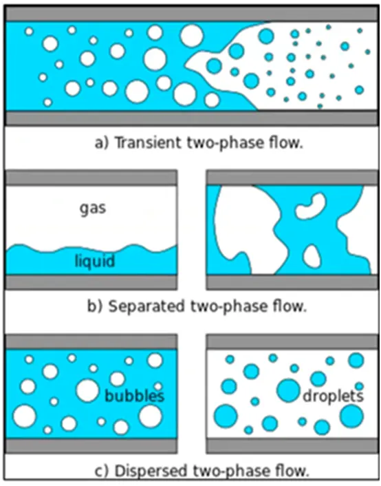
3.2. Different multiphase models :

• The most commonly used models in fluent as follows
  1. Volume of fluid
  2. Mixture models
  3. Eulereian model
  4. Wet steam model

1. Volume of fluid(VoF) model :

• The VOF model is a surface-tracking technique applied to a fixed Eulerian mesh.
• It is designed to find out the position of interface between the two or more immiscible fluids.
• The volume fraction of each fluid in each of the cell throughout domain can be tracked by using this method. And in this method single set of momentum equations is only shared by the fluids.
• In this method, all the control volumes must be filled with the single phase or combination of phases.
• This method is only applicable for pressure based solver.
• Applications of VOF model include stratified flows, free surface flows, filling, sloshing, the motion of large bubbles in a liquid, and the motion of liquid after a dam break, the prediction of jet breakup (surface tension), the steady or transient tracking of any liquid-gas interface.
• Let us consider, α₁- phase 1 and α₂ - phase 2

Then VOF should be α1 + α2= 1

2. Mixture models :

• Mixture models are used to model multiphase flow where the phases move at different velocities but assume local equilibrium over short spatial length.
• This method is applicable for liquid-solid flows and pressure based solver.
• It uses the concept of slip velocities to solve the different velocity phases.

3. Eulerian model :

• Eulerian model in ansys fluent allows for the modelling of multiple phases. The phases can be solids, liquids or gases. It can be in any of the combinations.
• Many number of secondary phases can be used in this model but it is limited only by the memory requirements and convergence behaviour.
• Here, the single pressure is only shared by all the phases.
• The limitation is that inviscid flow is not allowed in this model.

4. Wet steam model :

• Ansys has adopted the Eulerian-Eulerian approach for modelling the wet steam flow.
• The flow mixture is modelled using the compressible Navier-Stokes equations, in addition to two transport equations for the liquid-phase-mass-fraction, and the number of liquid droplets per unit volume.
• The phase change model, which involves the formation of liquid droplets in a homogeneous non-equilibrium condensation process, is based on the classical non-isothermal nucleation theory.
• In this model there is one term called maximum wetness model. It should not be set beyond 0.2.
• In this model we cannot change the properties of fluids because this model has some fixed properties of fluid. But we can change the properties of solids.
• This model is only applicable to the density based solver.

5. Difference between steady state and transient state analysis :

5.1. Steady state :

• In CFD simulations, a steady state is considered when all the flow properties like temperature, pressure, velocity are constant.
• Steady state simulation computes the fully developed solution that does not change w.r.t. time.
• When steady state is used mean values are computed.
• Steady state is always faster than the transient state simulations.

5.2. Transient state :

• Transient simulation computes the instantaneous values in each time for each quantity.
• Transient simulation has much higher requirements compared to steady-state like the CPU time, disk storage, evaluating results.
• Results of transient simulation may be more comprehensive than steady state analysis.
• There are 2 schemes are used in transient state
  1. Explicit scheme
  2. Implicit scheme

1. Explicit scheme :

• Explicit scheme is used for time dependent problems. In this method the volume fraction values are derived from the previous time step.

2. Implicit scheme :

• It will offer the speed of the steady state but we need a time-varying solution.
• It is unconditionally stable (timestep size is not a constraint) and is the default scheme in ansys fluent.
• Implicit scheme can be used for both steady and transient simulations.

5.3. In this challenge why transient analysis is preferred ? :

• Steady state simulation determines the fully developed solutions.
• Transient simulation, compared to steady state, has higher demand in terms of computational time, however transient solver better captures the flow and can be used to run at smaller time steps. Smaller time steps are required to observe the instabilities and can be only possible through transient simulation. Since it is a time marching solution, we expect more accuracy from transient simulation for which Transient simulation is the ideal setup to run the calculation for Rayleigh Taylor Instability.

6. Courant number :

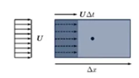
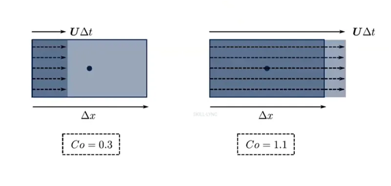
• It is a non-dimensional number that tells how fast information travels through our descretized domain.
• The Courant number is the ratio of these two lengths or fraction of the cell that the flow moves across in a time-step.
• For explicit time integration, the time step size must be less than a certain value or the solution would be false.
• Mathematically the courant number is given as,

`Co= ("Fluid distance")/("Cell distance") = (UDeltat)/(Deltax)`

Generally, CFL<1

Ex :

7. Atwood number :

• The Atwood number(A) is a dimensionless number in fluid dynamics used in the study of hydrodynamic instabilities in density stratified flows. It is a dimensionless density ratio defined as:

`A=(rho_1-rho_2)/(rho_1+rho_2)`

Where,

ρ₁ = density of heavier fluid

ρ₂ = density of lighter fluid

Modelling approach :

1. Pre-processing methods:

1.1. Geometry :

• Open ansys fluent
• Drag fluid flow(fluent) to project scheme
• Open the spaceclaim under geometry

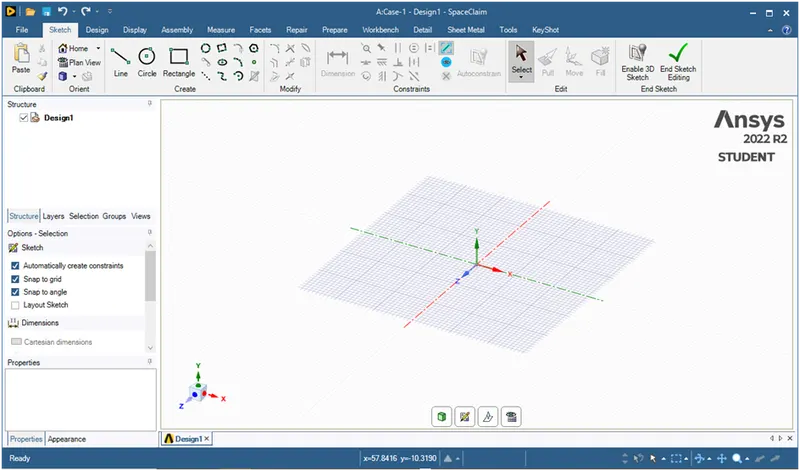
• Select sketch mode and select xy-plane
• Draw a rectangle of 20mm x 20mm by using rectangle tool from origin point.

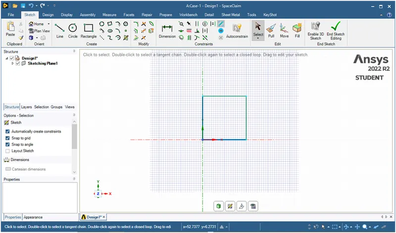
• Use pull tool to convert this sketch into surface.

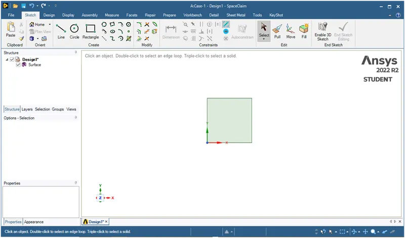
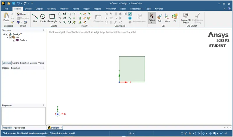
• Move this surface to new component by giving name as Air.

• Now again create a new component as water.
• Under this again draw a rectangle of same size above the previous rectangle.

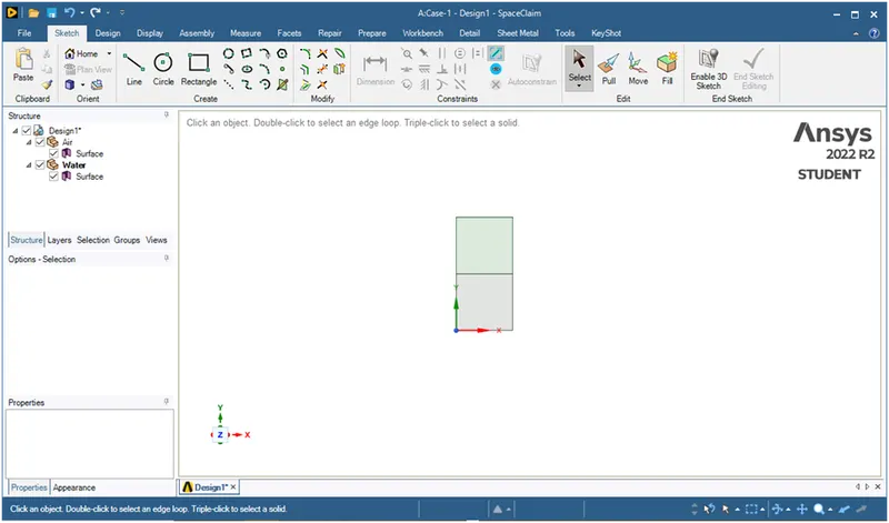
• Now we have done with geometry making.
• Now goto workbench and select share topology

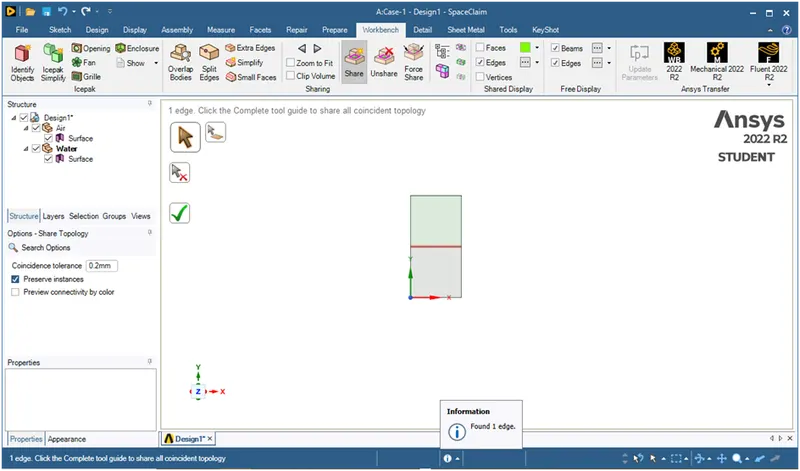
Now click on green tick.

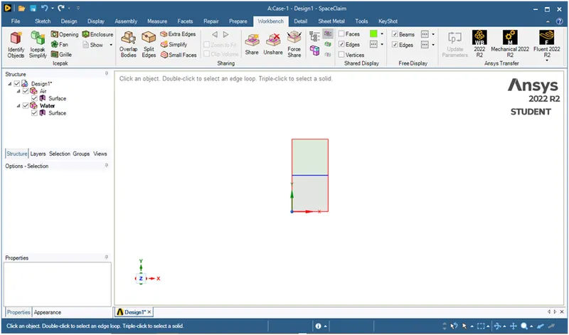
With this we are concluding the geometry cleanup. So lets go for meshing.

1.2. Meshing :

• Open mesh

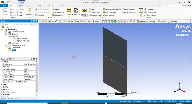
• Now here right click on mesh and then click on generate mesh

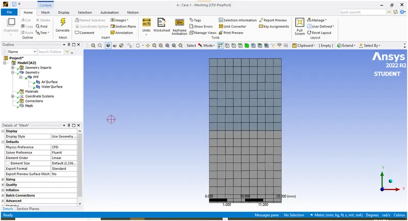
• Now according to problem statement for 1^st case we want mesh of 0.5mm so generate mesh of size 0.5mm.

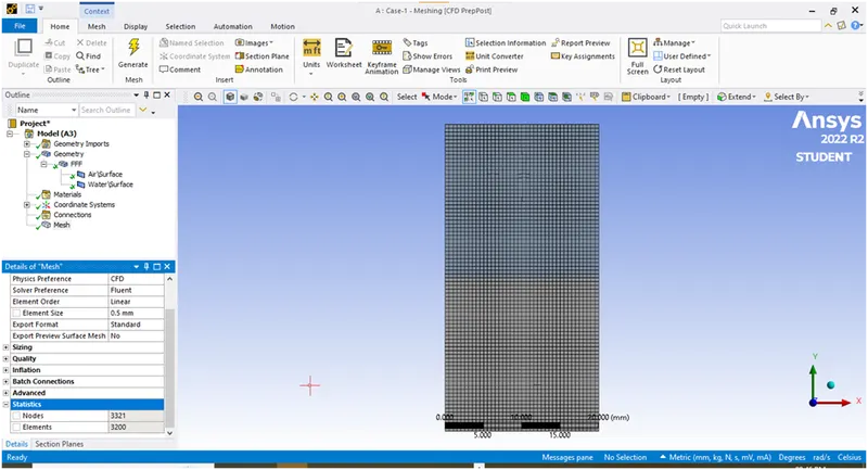
Now we have done with base line mesh.

• Now gives the name to the faces by selecting face selection mode as shows below.

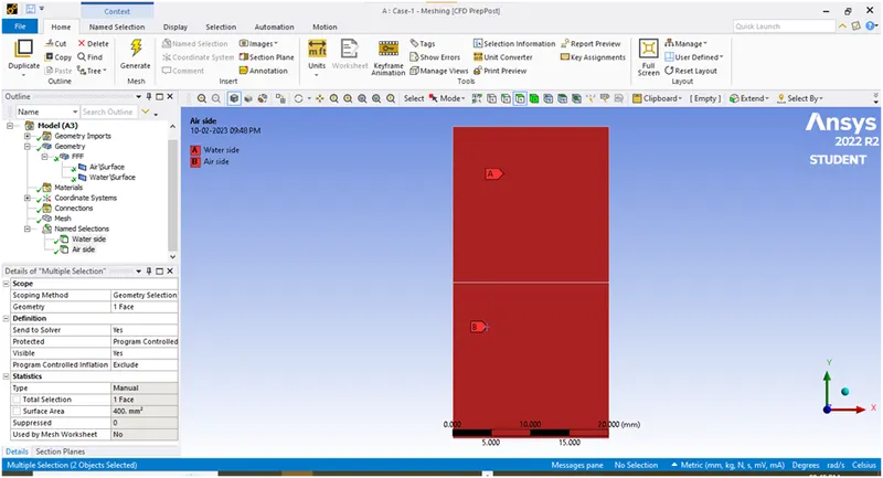
Now we have done with all. Just right click on mesh and then cick on update to transfer the data for post-processing.

2. Post-processing methods :

2.1. Setup :

• Open the ansys fluent

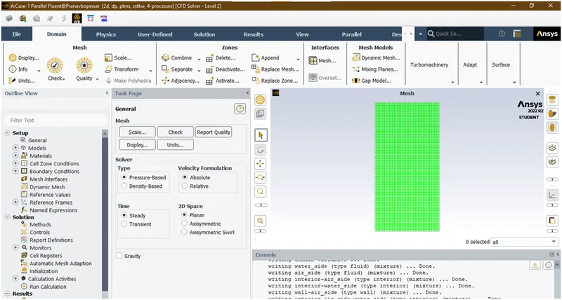
• Select transient and enabled gravity with -9.81m/s² as value in y-direction.
• Here I’m using pressure based solvers because here the velocity of fluid is very low here the mach no is less than 0.3. so it’s a incompressible fluid flow. So for incompressible fluid flow we are using pressure based solver and for compressible fluid flow i.e. Ma>0.3 we are using density based solvers.
• Then goto materials and add air and water from fluent database.

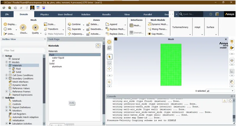
• Then goto models and select multiphase-VOF model with implicit scheme

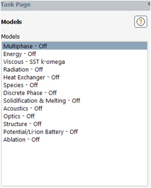
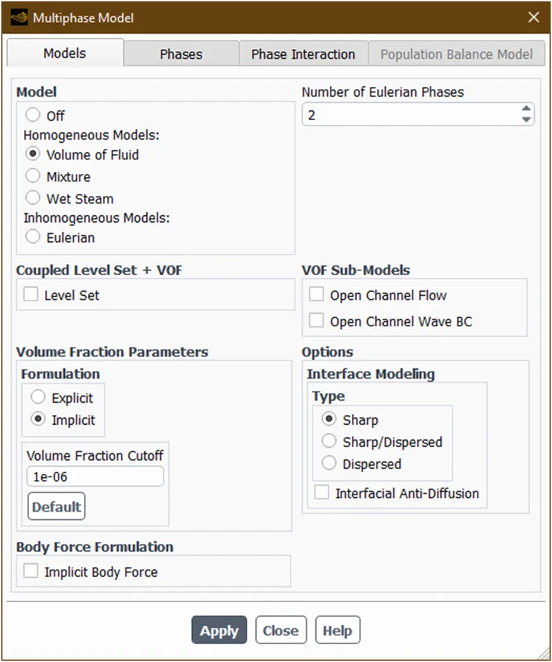
Click on apply and Then goto phases

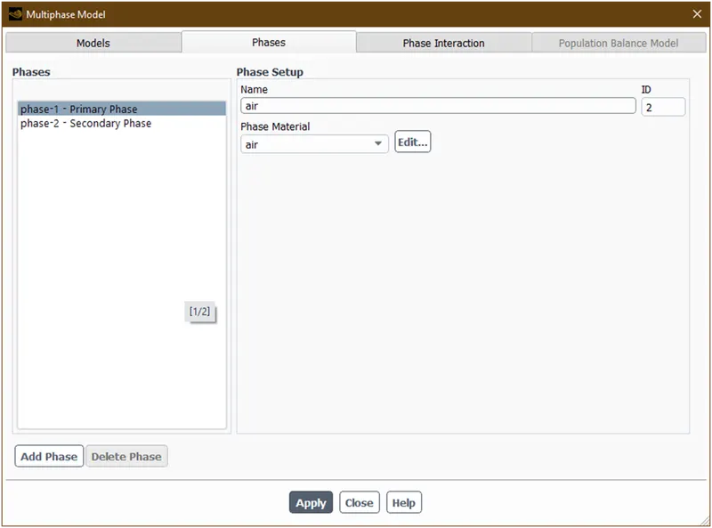
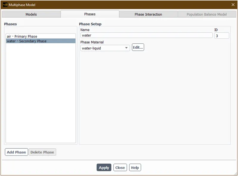
After adding phase just click on apply and then click on close.

• Now enabled viscous model as laminar model because we are not studied for force fluid.
• Select coupled method. Because coupled algorithm solves the continuity and momentum equations simultaneously. It takes less time to convergence. It solves all equations implicitily. It is a full implicit method.
• Now goto initialization and initialize the solution by standard initialization method

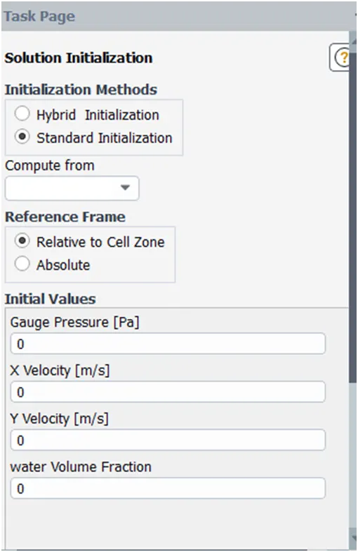
Scroll down

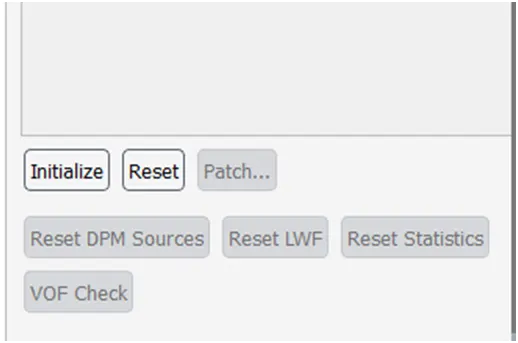
Now click on initialize.

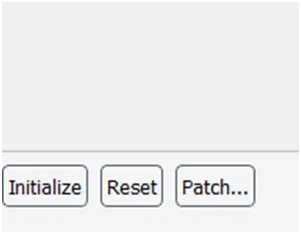
Click on patching

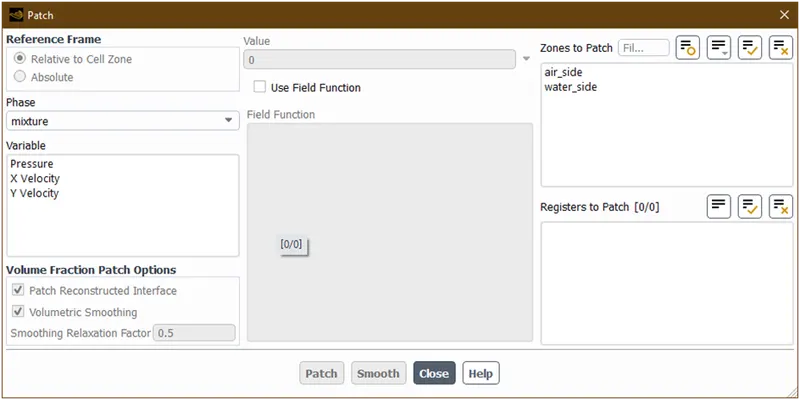
Now change the phases from mixture to water and patch the surface with given volume fraction as shown below

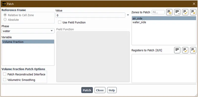
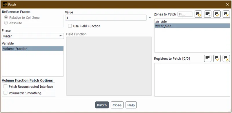
Now close.

• Now create one contour with phases and create an animation for this contour.
• Then run the solution for time step size 0.01s with number of steps=400
• After completing calculations save the animation.
• Now repeat the all process by changing the mesh size to 0.3mm for 2^nd case and save the animation.
• Again run the simulation for 3^rd case with 0.3mm mesh size and changing the material to user defined material with given properties and save the animation.

Results :

• Grid independent study

Sr.No	Mesh type	Mesh size	Cell counts	Animation
1	Course mesh	0.5mm	3200
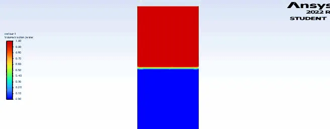2	Fine mesh	0.3mm	8978

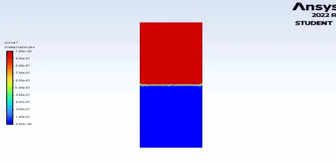• Difference between 2 cases with different fluid properties

Properties of fluids

1. Air-water(ρ_air =1.225, ρ_water =998.2)
2. UDF-water(ρ_UDF = 400kg/m³, ρ_water =998.2)

Sr.No	mixture	Atwood number	Animation
1	Air-Water	0.9975
2	UDF-Water	0.427

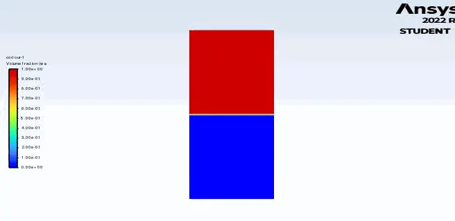• Residual plots

Sr.No	mixture	Mesh type	plots
1	Air-Water	Course mesh
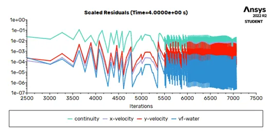2	Air-water	Fine mesh
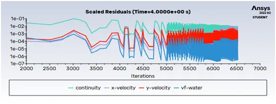3	UDF-Water	Fine mesh

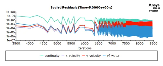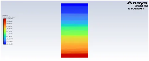
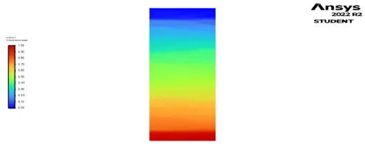
• Contour plots

Sr.No	mixture	Mesh type	plots
1	Air-Water	Course mesh
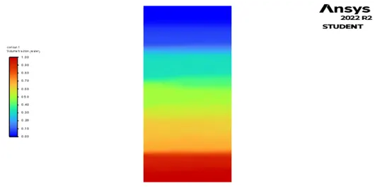2	Air-water	Fine mesh
3	UDF-Water	Fine mesh

Conclusions :

1. From mesh independent study, we can say that as we refining the mesh size we can see instability in fluids and mixing of fluids takes place very clearly and visible .Also as we refining the mesh size the computational time to solve the problem or simulate the problem has been increased. Also separation layers distance is different.
2. As Atwood number decreases means as we increase the density of one of the fluid, the mixing of fluids is not easy. As Atwood number near to 1 the mixing of fluid takes place very smoothly.
3. From residual plots we can say that after some iterations the solution has converged.