Week 5 - Rayleigh Taylor Instability

1. Practical CFD models that are based on mathematical analysis of rayleigh Taylor waves:

a) Kelvin–Helmholtz instability.
b) Richtmyer–Meshkov instability.
c) Plateau–Rayleigh instability.

a) Kelvin–Helmholtz instability:

The Kelvin–Helmholtz instability can occur when there is velocity shear in a single continuous fluid, or where there is a velocity difference across the interface between two fluids. An example is a wind blowing over water: The instability manifests in waves on the water surface.

b) Richtmyer–Meshkov instability:

The Richtmyer–Meshkov instability (RMI) occurs when two fluids of different density are impulsively accelerated. Normally this is by the passage of a shock wave. The development of the instability. begins with small amplitude perturbations which initially grow linearly with time. This is followed by a nonlinear regime with bubbles appearing in the case of a light fluid penetrating a heavy fluid, and with spikes appearing in the case of a heavy fluid penetrating a light fluid. A chaotic regime eventually is reached and the two fluids mix. This instability can be considered the impulsive-acceleration limit of the Richtmyer–Meshkov instability.

c) Plateau–Rayleigh instability:

The Plateau–Rayleigh instability, often just called the Rayleigh instability, explains why and how a falling stream of fluid breaks up into smaller packets with the same volume but less surface area. It is related to the Rayleigh-Taylor instability and is part of a greater branch of fluid dynamics concerned with fluid thread breakup. This fluid instability is exploited in the design of a particular type of ink-jet technology. whereby a jet of liquid is perturbed into a steady stream of droplets.

2) Objective :

We need to perform the Rayleigh Taylor instability simulation for 3 different mesh sizes with the base mesh being 0.5 mm. Also explaining why a steady-state approach might not be suitable for these types of simulation.

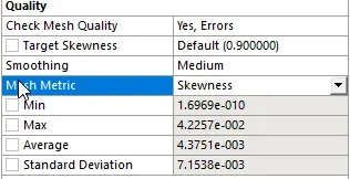
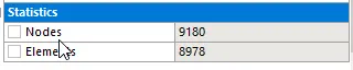
a) Meshes

a1) - Case 1 : 0.5 mm Mesh

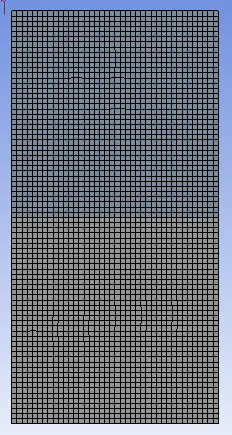
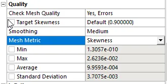
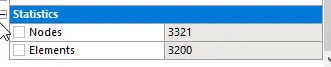
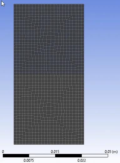
a2) - Case 2 : 0.3 mm Mesh

b) Solution Animations

b1) - Case 1 : 0.5 mm Mesh

b2) - Case 2 : 0.3 mm Mesh

c)Observation
Finer mesh captures the instability better than the coarse mesh , but it takes more time for the heavier fluid to settle down. So it is computationally expensive but produces results with better accuracy.

d)Why a steady-state approach might not be suitable for these types of simulation ?

Since the simulation involves capturing instabilities that are changing in an unpredictable manner as a function of time, the transient approach is preferred over the steady-state approach. More over our interest is in the timely development of the process since the final state is obviously known, i.e denser fluid at the bottom and lighter is on the top since the fluids are assumed to be immisible and non reactive.

3) Objective :

Here we have to do RT instability simulation with the refined mesh for with water and a user defined material of desnsity 400 kg/m3 and viscosity of  0.001 kg/m-s.

a) Mesh

b) solution Animation

 

4) Atwood Number:

• The Atwood number is a dimensionless number in fluid dynamics used in the study of hydrodynamic instabilities in density stratified flows.
• Atwood number is a dimensionless number that describes density difference between two adjacent fluids with a common interface.
• Atwood number is an important parameter in the study of Rayleigh–Taylor instability and Richtmyer–Meshkov instability.
• For Atwood number close to 0, RT instability flows take the form of symmetric “fingers” of fluid;
• for Atwood number close to 1, the much lighter fluid “below” the heavier fluid takes the form of larger bubble-like plumes.

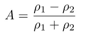
A	Atwood number (dimensionless)
ρ1	Density of heavier fluid (kg/m3)
ρ2	Density of lighter fluid. (kg/m3)

So Considering above Cases we can calculate the atwood number by using the above formula

So using the above formula we get Atwood NUmber as

Case 1 and Case 2 = 0.9955

Case 3 = 0.4285

The development of the R-t mixing region was characterized as a three-step process.

1. Originally, an exponential increase in infinitesimal fluctuations leading to linear stability analysis.
2. At a wavelength of roughly one-half, The instability is concentrated and the wavelength was longer(that have yet to reach saturation) take over. Emmons et al. (1960) also coined this regime's term ' bubble competition.
3. Ultimately, a self-similar R-T mixing layer with a scalar similarity is formed by nonlinear mode interaction and successive wavelength saturation gt^2

Behaviour of RT Instability on variation of Atwood number:

RTI evolves in three distinct stages: Linear stability , mushroom head(falling) or bubble(rising) formation , long term evolution due to bubble merging and mixing. For low Atwood number, bubble and mushroom head shape is relatively symmetrical, the disturbances or perturbations are linear for a larger time. In contrast, for large Atwood number, bubble and mushroom head shape is less symmetrical, also it occurs very rapidly at an accelerating rate which leads to a non linear growth rate.

5) Conclusion:

Atwood number forms a basis to compare and study research papers based on RT Instabilty. Thus we can use these papers to validate our results for beetter accuracy.