Analysis of quasi-one-dimensional flow through C-D nozzle using MacCormack method

Here we are going to simulate the isentropic flow through a quasi 1D subsonic-supersonic nozzle. We will be deriving both the conservation and non-conservation forms of the governing equations and solving them using the MacCormack's technique. Then we will define the steady-state flow-field. Also, we will compare the results from both the methods and study the difference between them. Computational Fluid Mechanics by Anderson is used for the reference.

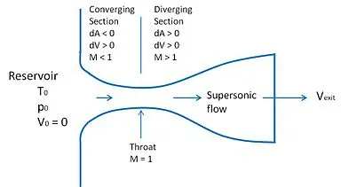
The above-given diagram shows a typical C-D Nozzle through which a supersonic flow can occur. The inlet of the nozzle is having a very large area and is connected to a reservoir having a very large size. In the tank, the fluid velocity is very very small since the mass flow rate is fixed. This is referred to as stagnation condition. When fluid starts moving through the nozzle since the flow is subsonic and is flowing through a converging section its velocity will increase. The throat is the section where there it has a minimum cross-sectional area. If the backpressure allows the speed of flow will become equal to the speed of sound at this section. Since the further part is a diverging section e may get a supersonic outflow depending upon the value of exit pressure. Here we are assuming that the values are constant radially and keep varying axially only. such a flow can be termed as quasi 1D flow.

Non-dimensionalization

For the convenience of study and analysis, there is a general practice of non-dimensionalization. For that, we will be dividing all the variable with reservoir values and area by throat area. So we can define non-dimensionalized parameters as follows.

`x' = x/L`

`rho' = rho/rho^o`

`T' = T/T^o`

`V' = V/a_o`

`t'= t/(L/a_o)`

`P=P/P^0`

`A'= A/A^"*"`

where,

L - Length of the Nozzle

`T^o , rho^o , P^o` - temperature, density and Pressure at the reservoir respectively.

`a_o = sqrt(gamma R T_o)` and

`A^"*"` - throat area.

now let's go to the governing equations.

MacCormack method

MacCormack method is a widely used discretization scheme for the numerical solution of hyperbolic partial differential equations. The MacCormack method is a variation of the two-step Lax–Wendroff scheme but is much simpler in the application. It's second-order accurate in both space and time. to employ second-order accuracy in time a predictor-corrector strategy is employed and their average is used to calculate the actual derivative. To illustrate the algorithm, consider the following first-order hyperbolic equation.

`frac(delu)(delt) + alpha*frac(delu)(delx) = 0`

First, we will be using a predictor formula to find out the value at the next time step. i.e.

`u_i^bar(n+1) = u_i^(n) - alpha* (Deltat)/(Deltax) *(u_(i+1)^(n) - u_i^(n))`

In the corrector step, the predicted value at the new time step is corrected according to the equation

`u_i^bar(n+1) = u_i^(n+(1)/2) - alpha* (Deltat)/(Deltax) *(u_(i)^bar(n+1) - u_(i-1)^bar(n+1))`

Replacing the `u_i^(n+(1)/2)` term by the temporal average will give

`u_i^(n+(1)/2) = (u_i^(n) + u_i^bar(n+1))/2`

to obtain the corrector step as

`u_i^(n+1) = (u_i^(n) + u_i^bar(n+1))/2 - alpha*(Deltat)/(2Deltax)*(u_i^bar(n+1) - u_(i-1)^bar(n+1))`

now let's go to the governing equations.

Governing Equations.

Conservation of mass momentum energy principle will give 3 Governing equations. Generally, a GE may be of two types, Conservative or non - conservative. here we will be solving the problem by using both the methods.

a) Non - Conservative form

Continuity equation

`A (del rho)/(del t) + V (del(rho A))/(del x) = -rho A (del V)/(del x)`

Momentum equation

`rho (del V)/(del t) + rho V(del V)/(del x) = -(del p)/(del x)`

Energy equation

`rho (del e)/(del t) + rho V(del e)/(del x) = - p(del V)/(del x) - pV(del(ln A))/(del x)`

up on non dimensiolization it will become as follows.

Continuity equation (non dimensional)

`(del rho')/(del t') = -rho' (del V')/(del x') - rho' V' (del (ln A'))/(del x') - V'(del rho')/(del x')`

Momentum equation (non dimensional)

`(del V')/(del t') = -V'(del V')/(del x') - 1/gamma((del T')/(del x') + (T')/(rho') (del rho')/(del x'))`

Energy equation (non dimensional)

`(del T')/(del t') = -V'(del T')/(del x') - (gamma-1)T'[(del V')/(del x') + V' (del(ln A'))/(del x')]`

Now we have to form the MacCromck Strategy.

Predictor Step

Find out time derivative at all the pints.

`((del rho)/(del t))_i^t = -rho_i^t[(V_(i+1)^t - V_i^t)/(Delta x)] - rho_i^t V_i^t[(ln(A_(i+1)) - ln(A_i))/(Delta x)] - V_i^t[(rho_(i+1)^t - rho_i^t)/(Delta x)]`

`((del V)/(del t))_i^t = -V_i^t[(V_(i+1)^t - V_i^t)/(Delta x)] - 1/gamma[(T_(i+1)^t - T_i^t)/(Delta x) + T_i^t/rho_i^t( (rho_(i+1)^t - rho_i^t)/(Delta x))]`

`((del T)/(del x))_i^t = -V_i^t[(T_(i+1)^t - T_i^t)/(Delta x)] - (gamma-1)T_i^t [(V_(i+1)^t-V_i^t)/(Delta x)+ V_i^t((ln(A_(i+1)) - ln(A_i))/(Delta x))]`

Compute Predicted values

`(bar rho)_i^(t+Delta t) = rho_i^t + ((del rho)/(del t))_i^t Delta t`

`(bar V)_i^(t+Delta t) = V_i^t + ((del V)/(del t))_i^t Delta t`

`(bar T)_i^(t+Delta t) = T_i^t + ((del T)/(del t))_i^t Delta t`

Corrector Step

Find time derivative values at time (t+dt) with the predicted values.

`(bar((del rho)/(del t)))_i^(t+Delta t) = -(bar rho)_i^(t+Delta t)[((bar V)_i^(t+ Delta t) - (bar V)_(i-1)^(t+Delta t))/(Delta x)] - (bar rho)_i^(t+Delta t)(bar V)_i^(t+Delta t)[(ln(A_i) - ln(A_(i-1)))/(Delta x)] - (bar V)_i^(t+Delta t)[((bar rho)_i^(t+Delta t) - (bar rho)_(i-1)^(t+Delta t))/(Delta x)]`

`(bar((del V)/(del t)))_i^(t+ Delta t) = -(bar V)_i^(t+Delta t)[((bar V)_i^(t+Delta t) - (bar V)_(i-1)^(t+Delta t))/(Delta x)] - 1/gamma[((bar T)_i^(t+Delta t) - (bar T)_(i-1)^(t+Delta t))/(Delta x) + (bar T)_i^(t+Delta t)/(bar rho)_i^(t+Delta t)( ((bar rho)_i^(t+Delta t) - (bar rho)_(i-1)^(t+Delta t))/(Delta x))]`

`(bar((del T)/(del x)))_i^(t+Delta t) = -(bar V)_i^(t+Delta t)[((bar T)_i^(t+Delta t) - (bar T)_(i-1)^(t+Delta t))/(Delta x)] - (gamma-1)T_i^(t+Delta t) [((bar V)_i^(t+Delta t)- (bar V)_(i-1)^(t+Delta t))/(Delta x)+ (bar V)_i^(t+Delta t)((ln(A_i) - ln(A_(i-1)))/(Delta x))]`

Find the average of time derivative values obtained from forward and backward difference methods.

`((del rho)/(del t))_(av) = 1/2[((del rho)/(del t))_i^t + (bar((del rho)/(del t)))_i^(t+Delta t)]`

`((del V)/(del t))_(av) = 1/2[((del V)/(del t))_i^t + (bar((del V)/(del t)))_i^(t+Delta t)]`

`((del T)/(del t))_(av) = 1/2[((del T)/(del t))_i^t + (bar((del T)/(del t)))_i^(t+Delta t)]`

Calculate the corrected values using the average value of time derivatives.

`rho_i^(t+Delta t) = rho_i^t + ((del rho)/(del t))_(av) Delta t`

`V_i^(t+Delta t) = V_i^t + ((del V)/(del t))_(av) Delta t`

`T_i^(t+Delta t) = T_i^t + ((del T)/(del t))_(av) Delta t`

`p_i^(t+Delta t) = rho_i^(t+Delta t) .T_i^(t+Delta t)`

Setting up

In Andersion Textbook shape of the nozzle is given by the following equation,

`A = 1 + 2.22*(x - 1.5)^2 0<= x <=3`

Initial Conditions are specified as

`rho = 1 - 0.3146 x`

`T = 1 - 0.2314 x`

`V = (0.1 + 1.09 x)T^(1/2)`

Given Boundary conditions are

Inlet

`V(1) = 2*V(2) - V(3)`

Outlet

`rho(n) = 2*rho(n-1) - rho(n-1)`
`V(n) = 2*V(n-1) - V(n-2)`
`T(n) = 2*T(n-1) - T(n-2)`

These things are used to code the Program.

b) Conservative form

For the quasi 1D subsonic-supersonic isentropic flow nozzle, the conservation form of the governing equations can be expressed as given below.

Continuity equation

`(del(rho A))/(del t) + (del(rho A V))/(del x) = 0`

Momentum equation

`(del(rho A V))/(del t) + (del(rho A V^2))/(del x) = -A (del p)/(del x)`

Energy equation

`(del[rho (e + V^2/2) A])/(del t) + (del[rho (e + V^2/2) VA])/(del x) = - (del(p A V))/(del x)`

Expressing the above equations in the dimensionless form

Continuity equation

`(del(rho' A'))/(del t') + (del(rho' A' V'))/(del x') = 0`

Momentum equation

`(del(rho' A' V'))/(del t') + (del[rho' A' V'^2 + (1/gamma)p'A'])/(del x') = 1/gamma p' (del A')/(del x')`

Energy equation

`(del T')/(del t') = -V'(del T')/(del x') - (gamma-1)T'[(del V')/(del x') + V' (del(ln A'))/(del x')]`

For the sake of simplicity in solving we can take U as solution vector, F as flux Vector and J as Source vector. then these equations can be represented as

`(del U_1)/(del t') = -(del F_1)/(del x')`
`(del U_2)/(del t') = J2 - (del F_2)/(del x')`
`(del U_3)/(del t') = -(del F_3)/(del x')`

where

`U_1 = rho' A'`
`U_2 = rho' A' V'`
`U_3 = rho'((e')/(gamma-1)+gamma/2 V'^2)A'`
`F_1 = rho' A' V'`
`F_2 = rho' A' V'^2 + 1/gamma p'A'`
`F_3 = rho'((e')/(gamma-1) + gamma/2 V'^2)V' A' + p' A' V'`
`J_2 = 1/gamma p' (del A')`

While writing the code, we'll solve for the solution vectors and then consecutively calculate the primitive variables using the following relations.

`rho' = (U')/(A')`

`V' = U_2/U_1`

`T' = e' = (gamma-1)(U_3/U_1-gamma/2 V'^2)`

`p' = rho' T'`

W have to solve the solution vectors.flux terms and source terms must also be expressed in terms of U1, U2 and U3 to obtain the pure form of the flux terms.

`F_1 = U_2`

`F_2 = U_2^2/U_1 + (gamma-1)/gamma(U_3 - gamma/2 U_2^2/U_1)`

`F_3 = gamma (U_2 U_3)/U_1 - (gamma(gamma-1))/2 U_2^3/U_1^2`

`J_2 = (gamma-1)/gamma(U_3 - gamma/2 U_2^2/U_1)(del(ln A'))/(del x')`

now we have to apply the MacCromack Method here.

Predictor step

Calculate timederivative of quantities.

`((del U_1)/(del t'))_i^t = -(F_(1(i+1))^t - F_(1(i))^t)/(Delta x')`

`((del U_2)/(del t'))_i^t = (J_(2(i+1))^t-J_(2(i))^t)/(Delta x') - (F_(2(i+1))^t - F_(2(i))^t)/(Delta x')`

`((del U_3)/(del t'))_i^t = -(F_(3(i+1))^t - F_(3(i))^t)/(Delta x')`

Compute Predicted values

`bar(U)_(1(i))^(t+Delta t) = ((del U_1)/(del t'))_i^t .Delta t'`

`bar(U)_(2(i))^(t+Delta t) = ((del U_2)/(del t'))_i^t .Delta t'`

`bar(U)_(3(i))^(t+Delta t) = ((del U_3)/(del t'))_i^t .Delta t'`

Corrector Step

Find time derivative values at time (t+dt) with the predicted values.

`(bar(del U_1)/(del t'))_i^(t+Delta t) = -(bar(F)_(1(i))^(t+Delta t) - bar(F)_(1(i-1))^(t+Delta t))/(Delta x')`

`(bar(del U_2)/(del t'))_i^(t+Delta t) = (bar(J)_(2(i))^(t+Delta t)-bar(J)_(2(i-1))^(t+Delta t))/(Delta x') - (bar(F)_(2(i))^(t+Delta t) - bar(F)_(2(i-1))^(t+Delta t))/(Delta x')`

`(bar(del U_3)/(del t'))_i^(t+Delta t) = -(bar(F)_(3(i))^(t+Delta t) - bar(F)_(3(i-1))^(t+Delta t))/(Delta x')`

Find the average of time derivative values obtained from forward and backward difference methods.

`((del U_1)/(del t'))_(av)=1/2[((del U_1)/(del t'))_i^t+(bar(del U_1)/(del t'))_i^(t+Delta t)]`

`((del U_2)/(del t'))_(av)=1/2[((del U_2)/(del t'))_i^t+(bar(del U_2)/(del t'))_i^(t+Delta t)]`

`((del U_3)/(del t'))_(av)=1/2[((del U_3)/(del t'))_i^t+(bar(del U_3)/(del t'))_i^(t+Delta t)]`

Calculate the corrected values using the average value of time derivatives.

`U_(1(i))^(t+Delta t) = ((del U_1)/(del t'))_(av) .Delta t'`

`U_(2(i))^(t+Delta t) = ((del U_2)/(del t'))_(av).Delta t'`

`U_(3(i))^(t+Delta t) = ((del U_3)/(del t'))_(av).Delta t'`

Setting up

In Andersion Textbook shape of the nozzle is given by the following equation,

`A = 1 + 2.22*(x - 1.5)^2 0<= x <=3`

The conservation form is much sensitive to initial conditions so, we will be applying the following initial condition.

`0<=x'<=0.5 {(rho',=,1),(T',=,1):}`

`0.5<=x'<=1.5 {(rho',=,1-0.366(x'-0.5)),(T',=,1-0.167(x'-0.5)):}`

`1.5<=x'<=3 {(rho',=,0.634-0.3879(x'-1.5)),(T',=,0.833-0.3507(x'-1.5)):}`

The variation of Velocity for initial conditions can be introduced by mass flow (U2) condition. If we are choosing U2 = 0.59 for initial condition, then

`V' = U_2/(rho' A')`

The same initial conditions should be be applied to U1, U2 and U3. for that following relations can be used.

`U_1 = rho' A'`

`U_2 = rho' A' V' = 0.59`

`U_3 = rho'((e')/(gamma-1)+gamma/2 V'^2)A'`

Given Boundary conditions are

Inlet

`U_1(1) = rho'(1) *A'(1)`

`U_2(1) = 2 U_2(2) - U_2(3)`

`V'(1) = (U_2(1))/(rho'(1)*A'(1))`

`U_3(1) = U_1(1)((T'(1))/(gamma-1) + gamma/2 V'(1)^2)`

Outlet

`U1(1) = 2*U1(n-1) - U1(n-2)`

`U2(1) = 2*U2(n-1) - U2(n-2)`

`U3(1) = 2*U3(n-1) - U3(n-2)`

These things are used to code the Program.

MATLAB Code

clear all
close all
clc

% Inputs
n = 31;
L = 3;
x = linspace(0, L, n);
dx = x(2) - x(1);
nt =1400;
% Specific Heat
gamma = 1.4;

% Courant Number
C = 0.5;

% Area Profile
A = 1 + 2.2*(x - 1.5).^2;

% Throat Index
n_throat = find(A == min(A));

for solver = 1:2
    % Non - Conservative Solver

if solver == 1

    % Calculate Initial Profile

    rho = 1 - 0.3146*x;
    T = 1 - 0.2314*x;
    v = (0.1 + 1.09*x) .* T.^0.5;

    % Non - Conservative Solver Function
    [rho_nc, v_nc, T_nc, P_nc, M_nc, mass_flow_nc,dtnc,rho_tnc,p_tnc, v_tnc, T_throatnc,M_tnc] = non_conservative_function_MacCormack(n,x,dx, gamma, A, rho, v, T, C,nt,n_throat);
end


% Conservative Solver

if solver == 2

    % Initial Profiles
    % Density & Temperature

        for k = 1: n

                if x(k) >= 0 && x(k) < 0.5
                        rho(k) = 1;
                        T(k) = 1;

                elseif x(k) >= 0.5 && x(k) < 1.5

                        rho(k) = 1 - 0.366 * (x(k) - 0.5);
                        T(k) = 1 - 0.167 * (x(k) - 0.5);

                 elseif x(k) >= 1.5 && x(k) <= 3

                        rho(k) = 0.634 - 0.3879 * (x(k) - 1.5);
                        T(k) = 0.833 - 0.3507 * (x(k) - 1.5);
                end
        end

    % Velocity
    v = 0.59 ./ (rho .* A);

    % Conservative Solver Function
    [rho_c, v_c, T_c, P_c, M_c, mass_flow_c,dtc,rho_tcf,p_tcf, v_tcf, T_throatcf,M_tcf] = conservative_function_MacCormack(n,x, dx,gamma, A, rho, v, T, C,nt,n_throat);
   
end
end

%%
%Plotting Non dimensionalized primitive variables Non conservative
figure(3)
opengl software
plot(x,rho_nc,'m', 'linewidth', 1.5)
grid minor
hold on
plot(x,v_nc,'r', 'linewidth', 1.5)
hold on
plot(x,T_nc,'k', 'linewidth', 1.5)
hold on
plot(x,P_nc,'c', 'linewidth', 1.5)
title('Steady state distribution of primitive variables - non conservative form')
legend("(rho/rho_0)","(v/v_0)","(T/T0)","(P/P_0)",'Location','Best')
xlabel ('X')
ylabel('Non - dimensional primitive variable')
%%
figure(4)
subplot(2,2,1)
nozGrid(x,A,v_nc);
title(sprintf("Variation of non dimensional velocity along the axis at steady state \n non - conservative form"))

subplot(2,2,2)
nozGrid(x,A,rho_nc);
title(sprintf("Variation of non dimensional density along the axis at steady state \n non - conservative form"))

subplot(2,2,3)
nozGrid(x,A,P_nc);
title(sprintf("Variation of non dimensional Pressure along the axis at steady state \n non - conservative form"))

subplot(2,2,4)
nozGrid(x,A,T_nc);
title(sprintf("Variation of non dimensional Temparature along the axis at steady state \n non - conservative form"))


%%
%Plotting Non dimensionalized primitive variables conservative
figure(5)
opengl software
plot(x,rho_c,'m', 'linewidth', 1.5)
grid minor
hold on
plot(x,v_c,'r', 'linewidth', 1.5)
hold on
plot(x,T_c,'k', 'linewidth', 1.5)
hold on
plot(x,P_c,'c', 'linewidth', 1.5)
title('Steady state distribution of primitive variables - Conservative form')
legend("(rho/rho_0)","(v/v_0)","(T/T0)","(P/P_0)",'Location','Best')
xlabel ('X')
ylabel('Non - dimensional primitive variable')
%%
figure(6)
subplot(2,2,1)
nozGrid(x,A,v_c);
title(sprintf("Variation of non dimensional velocity along the axis at steady state \n conservative form"))

subplot(2,2,2)
nozGrid(x,A,rho_c);
title(sprintf("Variation of non dimensional density along the axis at steady state \n conservative form"))

subplot(2,2,3)
nozGrid(x,A,P_c);
title(sprintf("Variation of non dimensional Pressure along the axis at steady state \n conservative form"))

subplot(2,2,4)
nozGrid(x,A,T_c);
title(sprintf("Variation of non dimensional Temparature along the axis at steady state \n conservative form"))

%%

timenc = dtnc*nt;
t_NC = [dtnc:dtnc:timenc];

figure(7)
plot(t_NC,rho_tnc)
grid minor
hold on
plot(t_NC,p_tnc)
hold on
plot(t_NC,v_tnc)
hold on
plot(t_NC,T_throatnc)
hold on
plot(t_NC,M_tnc)
xlabel('Time')
ylabel('Non-dimensional Variables')
title(sprintf("Variation of Variables with time \n non-conservative form"))
legend("rho/rho_0","P/P_0","V/V_0","T/T0","Mach Number")

%%
timecf = dtc*nt;
t_CF = [dtc:dtc:timecf];

figure(8)
plot(t_CF,rho_tcf)
grid minor
hold on
plot(t_CF,p_tcf)
hold on
plot(t_CF,v_tcf)
hold on
plot(t_CF,T_throatcf)
hold on
plot(t_CF,M_tcf)
xlabel('Time')
ylabel('Non-dimensional Variables')
title(sprintf("Variation of Variables with time \n conservative form"))
legend("rho/rho_0","P/P_0","V/V_0","T/T0","Mach Number")
%%
figure(9)
plot(x,mass_flow_c,'m', 'linewidth', 1.5)
grid minor
hold on
plot(x,mass_flow_nc,'b', 'linewidth', 1.5)
legend('Conservative form','Non Conservative form')
title('Mass flow rate in Conservative form & Non Conservative form')
xlabel('X')
ylabel('Normalized mass flow rate')

MATLAB function for conservative form

function [rho, v, T, P, M, mass_flow,dtc,rho_t,p_t, v_t, T_throat,M_t] = conservative_function_MacCormack(n,x,dx, gamma, A, rho, v, T, C, nt,n_throat)
   
    % Solution Vectors
    U1 = rho .* A;
    U2 = rho .* A .* v;
    U3 = rho .* (T/(gamma-1) + (gamma/2) * (v.^2)) .* A;
    
    % Time step based on Stability
    a = sqrt(T);
    delt = (C * dx) ./ (a + v);
    dt = min(delt);
    dtc = dt;

    % Initializing Loop
    for z = 1:nt 
        U1_old = U1;
        U2_old = U2;
        U3_old = U3;
        
        % Flux Vectors
        F1 = U2;
        F2 = (U2.^2 ./ U1) + ((gamma-1)/gamma) * (U3 - (gamma/2) * (U2.^2 ./ U1));
        F3 = (gamma * ((U2 .* U3) ./ U1)) - (gamma*(gamma-1)/2) * (U2.^3 ./ U1.^2);


        % Predictor Step  (FDS)
        for i = 2: n-1
            dF1_dx = (F1(i+1) - F1(i)) / dx;
            dF2_dx = (F2(i+1) - F2(i)) / dx;
            dF3_dx = (F3(i+1) - F3(i)) / dx;
            dA_dx = (A(i+1) - A(i)) / dx;

            % Source Term
            J2(i) = (1/gamma) * rho(i) * T(i) * dA_dx;

            % Continuity Equation
            dU1_dt_p(i) = -dF1_dx;

            % Momentum Equation
            dU2_dt_p(i) = -dF2_dx + J2(i);

            % Energy Equation
            dU3_dt_p(i) = -dF3_dx;


            % Solution Update
            U1(i) = U1(i) + dU1_dt_p(i) * dt;
            U2(i) = U2(i) + dU2_dt_p(i) * dt;
            U3(i) = U3(i) + dU3_dt_p(i) * dt;

        end


       % Update Flux Vectors

        F1 = U2;
        F2 = (U2.^2 ./ U1) + ((gamma-1)/gamma) * (U3 - (gamma/2) * (U2.^2 ./ U1));
        F3 = (gamma * ((U2 .* U3) ./ U1)) - (gamma*(gamma-1)/2) * (U2.^3 ./ U1.^2);    


        % Update Flow Properties to apply in source term

        rho = U1 ./ A;
        v = U2 ./ U1;
        T = (gamma - 1) * (U3 ./ (rho .* A) - (gamma/2) * v.^2);

        % Corrector step  (BDS)

        for i = 2: n-1

            dF1_dx = (F1(i) - F1(i-1)) / dx;
            dF2_dx = (F2(i) - F2(i-1)) / dx;
            dF3_dx = (F3(i) - F3(i-1)) / dx;
            dA_dx = (A(i) - A(i-1)) / dx;

            % Source Term
            J2(i) = (1/gamma) * rho(i) * T(i) * dA_dx;

            % Continuity Equation
            dU1_dt_c(i) = -dF1_dx;

            % Momentum Equation
            dU2_dt_c(i) = -dF2_dx + J2(i);

            % Energy Equation
            dU3_dt_c(i) = -dF3_dx;

        end

        % Compute the Average Derivative

        dU1_dt = 0.5 * (dU1_dt_p + dU1_dt_c);
        dU2_dt = 0.5 * (dU2_dt_p + dU2_dt_c);
        dU3_dt = 0.5 * (dU3_dt_p + dU3_dt_c);


        % Final Solution update

        for j = 2: n-1

            U1(j) = U1_old(j) + dU1_dt(j) * dt;
            U2(j) = U2_old(j) + dU2_dt(j) * dt;
            U3(j) = U3_old(j) + dU3_dt(j) * dt;

        end

        % Apply Boundary Conditions

        % Inlet
        rho(1) = 1;
        T(1) = 1;

        U1(1) = rho(1) * A(1);
        U2(1) = 2 * U2(2) - U2(3);
        U3(1) = U1(1) * (T(1)/(gamma-1) + (gamma/2) * ((U2(1) / U1(1))^2));

        % Outlet
        U1(n) = 2 * U1(n-1) - U1(n-2);
        U2(n) = 2 * U2(n-1) - U2(n-2);
        U3(n) = 2 * U3(n-1) - U3(n-2);

        % Update Flow Properties
        rho = U1 ./ A;
        v = U2 ./ U1;
        T = (gamma - 1) * (U3 ./ (rho .* A) - (gamma/2) * v.^2);
        P = rho .* T;
        M = v ./ sqrt(T);
        mass_flow = rho .* v .* A;
        
        %Storing values at the throat
        rho_t(z)=rho(n_throat);
        p_t(z)=P(n_throat);
        v_t(z)=v(n_throat);
        T_throat(z)=T(n_throat);
        M_t(z) = M(n_throat);  
        
        figure(2);        
        if z == 1
            plot(x, mass_flow, '--k', 'linewidth', 1.5)
            grid minor
            hold on
        elseif z == 50
            plot(x, mass_flow, 'r', 'linewidth', 1.5)
            hold on
        elseif z == 100
            plot(x, mass_flow, 'b', 'linewidth', 1.5)
            hold on
        elseif z == 150
            plot(x, mass_flow, 'g', 'linewidth', 1.5)
            hold on
        elseif z == 200
            plot(x, mass_flow, 'm', 'linewidth', 1.5)
            hold on
        elseif z == nt
            plot(x, mass_flow, '-.k', 'linewidth', 2)
            xlabel('x')
            ylabel('Mass Flow')
            legend('1Deltat', '50Deltat', '100Deltat', '150Deltat', '200Deltat', 'Steady State','Location','Best')
            title(sprintf('Transient State Mass Flow Profile for Conservative Solver'))
            hold off   
        end
        
        
        
    end
 

            
end

MATLAB function for non - conservative form

function [rho, v, T, P, M, mass_flow,dtnc,rho_t,p_t, v_t, T_throat,M_t] = non_conservative_function_MacCormack(n,x,dx, gamma, A,rho,v, T, C,nt,n_throat)
        
    for z = 1:nt
               
        rho_old = rho;
        v_old = v;
        T_old = T;
        
        % Time step based on Stability        
        a_old = sqrt(T_old);
        delt = (C * dx) ./ (a_old + v_old);
        dt = min(delt);
        dtnc=dt;

        % Predictor Step  (FDS)

        for i = 2: n-1

            drho_dx = (rho(i+1) - rho(i)) / dx;
            dv_dx = (v(i+1) - v(i)) / dx;
            dT_dx = (T(i+1) - T(i)) / dx;
            dlogA_dx = (log(A(i+1)) - log(A(i))) / dx;

            % Continuity Equation
            drho_dt_p(i) = -(rho(i) * dv_dx) - (rho(i) * v(i) * dlogA_dx) - (v(i) * drho_dx);

            % Momentum Equation
            dv_dt_p(i) = -(v(i) * dv_dx) - (1/gamma) * (dT_dx + (T(i)/rho(i)) * drho_dx);

            % Energy Equation
            dT_dt_p(i) = -(v(i) * dT_dx) - (gamma - 1) * T(i) * (dv_dx + v(i) * dlogA_dx);

            % Solution Update
            rho(i) = rho(i) + drho_dt_p(i) * dt;
            v(i) = v(i) + dv_dt_p(i) * dt;
            T(i) = T(i) + dT_dt_p(i) * dt;

        end

        % Corrector Step  (BDS)

        for i = 2: n-1

            drho_dx = (rho(i) - rho(i-1)) / dx;
            dv_dx = (v(i) - v(i-1)) / dx;
            dT_dx = (T(i) - T(i-1)) / dx;
            dlogA_dx = (log(A(i)) - log(A(i-1))) / dx;

            % Continuity Equation
            drho_dt_c(i) = -(rho(i) * dv_dx) - (rho(i) * v(i) * dlogA_dx) - (v(i) * drho_dx);

            % Momentum Equation
            dv_dt_c(i) = -(v(i) * dv_dx) - (1/gamma) * (dT_dx + (T(i)/rho(i)) * drho_dx);

            % Energy Equation
            dT_dt_c(i) = -(v(i) * dT_dx) - (gamma - 1) * T(i) * (dv_dx + v(i) * dlogA_dx);

        end

        % Compute the Average Derivative

        drho_dt = 0.5 * (drho_dt_p + drho_dt_c);
        dv_dt = 0.5 * (dv_dt_p + dv_dt_c);
        dT_dt = 0.5 * (dT_dt_p + dT_dt_c);

        % Final Solution update

        for j = 2: n-1

            rho(j) = rho_old(j) + drho_dt(j) * dt;
            v(j) = v_old(j) + dv_dt(j) * dt;
            T(j) = T_old(j) + dT_dt(j) * dt;

        end

        % Apply Boundary Conditions

        % Inlet
        
        v(1) = 2 * v(2) - v(3);
        

        % Outlet
        rho(n) = 2 * rho(n-1) - rho(n-2);
        v(n) = 2 * v(n-1) - v(n-2);
        T(n) = 2 * T(n-1) - T(n-2);
        
        P = rho .* T;
        M = v ./ sqrt(T);
        mass_flow = rho .* v .* A;
        
        rho_t(z)=rho(n_throat);
        p_t(z)=P(n_throat);
        v_t(z)=v(n_throat);
        T_throat(z)=T(n_throat);
        M_t(z) = M(n_throat);   
        
        
        
        % Plotting the Transient Mass Flow Rate
        figure(1);        
        if z == 1
            plot(x, mass_flow, '--k', 'linewidth', 1.5)
            grid minor
            hold on
        elseif z == 50
            plot(x, mass_flow, 'r', 'linewidth', 1.5)
            hold on
        elseif z == 100
            plot(x, mass_flow, 'b', 'linewidth', 1.5)
            hold on
        elseif z == 150
            plot(x, mass_flow, 'g', 'linewidth', 1.5)
            hold on
        elseif z == 200
            plot(x, mass_flow, 'm', 'linewidth', 1.5)
            hold on
        elseif z==nt
            plot(x, mass_flow, '-.k', 'linewidth', 2)
            xlabel('x')
            ylabel('Mass Flow')
            legend('1Deltat', '50 Deltat', '100 Deltat', '150 Deltat', '200 Deltat', 'Steady State','Location','Best')
            title(sprintf('Transient State Mass Flow Profile for Non - Conservative Solver'))
            hold off
        end

    end
 

    

end

MATLAB function for flow visualization

function [a,b] = nozGrid(x,AA,v)
y = linspace(-max(AA), max(AA), length(x));
vplot = ones(length(x),length(y));
for i = 1: length(x)
	for j = 1 : length (y)        
		if abs(y(j))<AA(i)
            vplot(i,j) = v(i);
        else
            vplot(i,j) = -0.1;
        end         
	end
end

[a,b] = contourf(x,y,vplot','showText','off');
% colorbar;
colormap(jet);clc
xlabel('X Axis');
title(sprintf('Variation of non-dimensional velocity along the axial direction \n non - Conservative Form. Number of node = 201'))
ylabel('Y Axis');
hold on
plot(x,AA,'w','linewidth', 2)
hold on
plot(x,-AA,'w','linewidth', 2)
end

Results

1. Steady-state distribution of primitive variables inside the nozzle

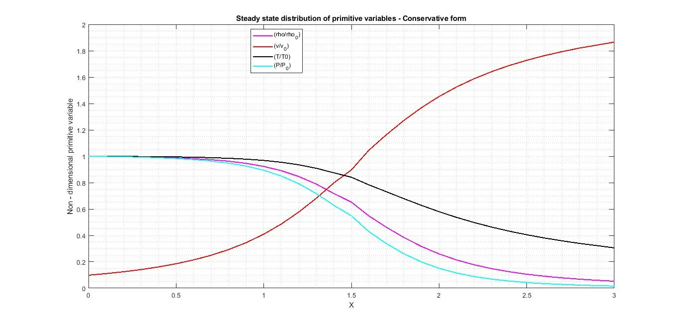
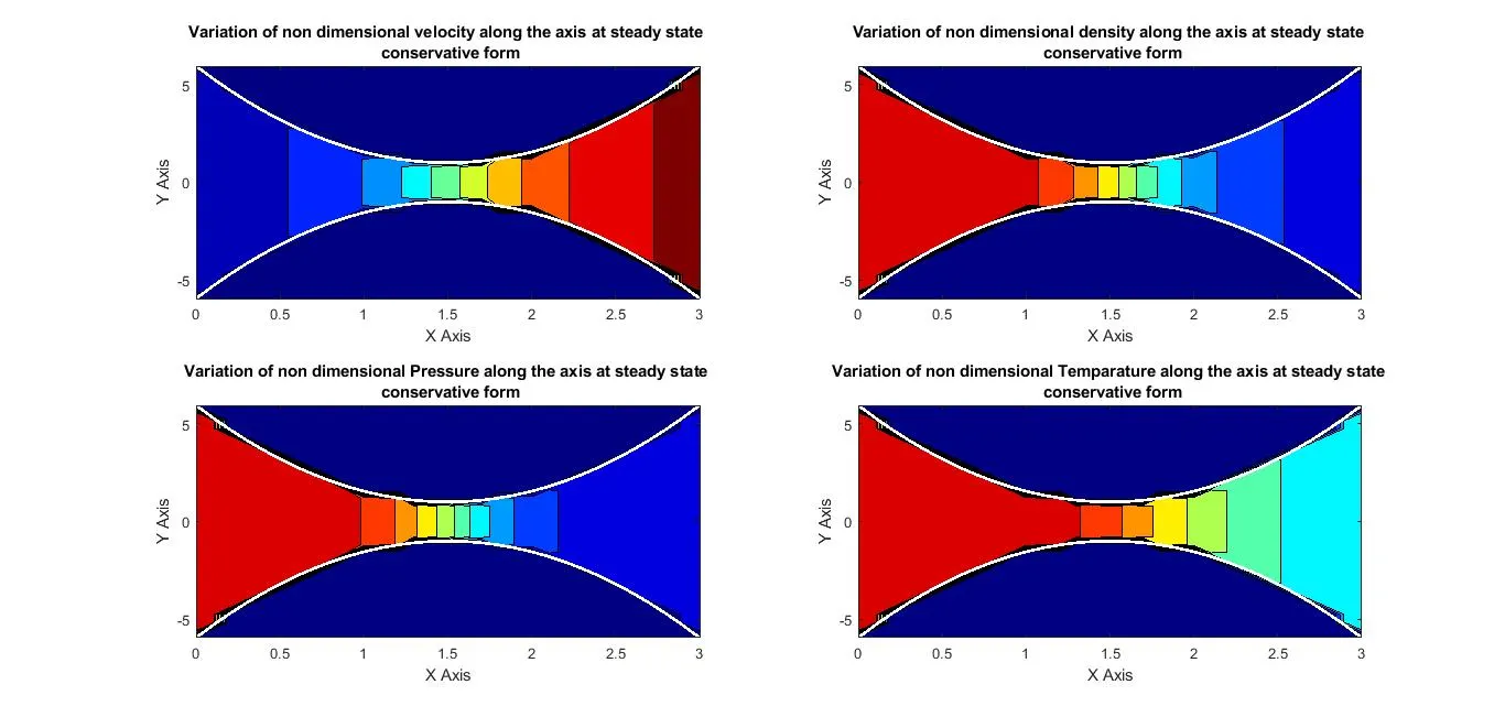
a)Conservative form

The Steady-state distribution of various primitive variables obtained via the conservative form of the equations is shown here. The Trend is verified by referring Anderson Textbook

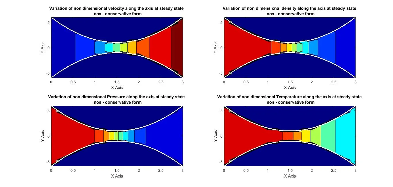
b)Non - Conservative form

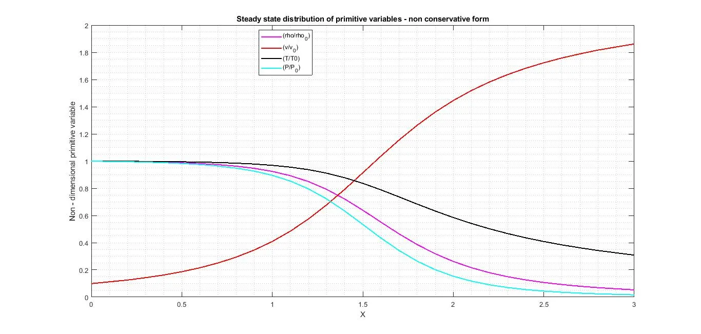
The Steady-state distribution of various primitive variables obtained via the non-conservative form of the equations is shown here. The Trend is verified by referring Anderson Textbook

2. Time-wise variation of the primitive variables

a) Conservative form

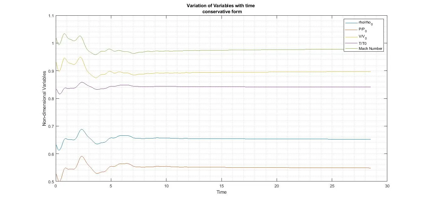
The below figure shows the time-wise variation of various primitive values at the throat using conservative method.

b)Non - Conservative form

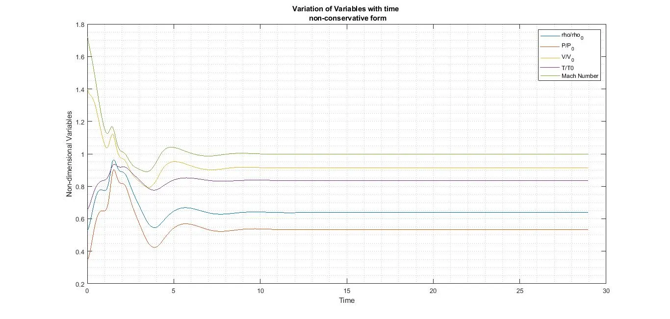
The below figure shows the time-wise variation of various primitive values at the throat using the non-conservative method

3. Variation of Mass flow rate distribution inside the nozzle at different time steps during the time-marching process

a) Conservative form

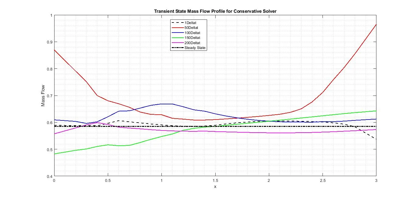
Time-wise variation of mass flow along with the axis is plotted here. Here the conservative form is used

b)Non - Conservative form

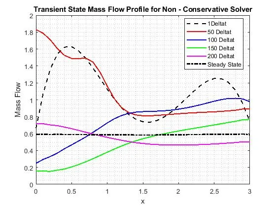
Time-wise variation of mass flow along with the axis is plotted here. Here the non-conservative form is used

4. Comparison of Normalized mass flow rate distributions of both forms.

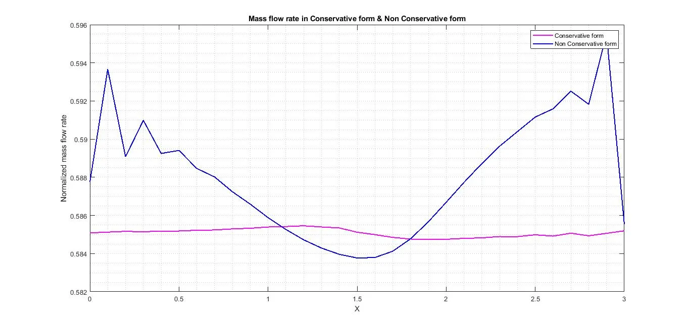
The steady-state mass-flow rate obtained via both forms of the equations is plotted here.

Grid Independence Test.

The above code is run for double the number of nodes and the final distribution is almost a constant. So the solution is grid-independent.

I am attaching my code below.