Central and Skewed stencil-based derivation of second derivative having order of truncation error of the order of four by using Taylors table method.

Central Difference method

To obtain a fourth order truncation error we have to take 4 points other than the point of interest. Two of them are at right and two of them are left. The stencil representing the condition is shown below.

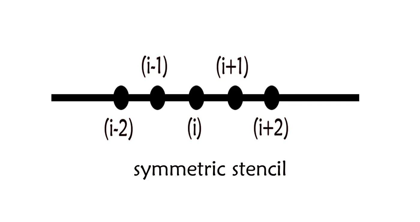
We will be deriving the formula for second order derivative having a truncation error of the order 4 by using these 5 points (2+4-1 = 5).

First, we assume that

`(d^2f)/(dx^2) = a*f(i-2) + b*f(i-1) + c*f(i) + d*f(i+1) + e*f(i+2)`

Now our job is to find the values of a, b, c, d and e. for that we will be using the method of Taylors table.

	f(i)	f’(i) *ΔX	f’’(i) *ΔX2	f’’’(i) *ΔX3	f’’’’(i) *ΔX4	f’’’’’(i) *ΔX5	f’’’’’(i) *ΔX5
a * f(i-2)	a	-2a	2a	`(-8*a)/6`	`(16*a)/24`	`(-32*e)/120`	`(64*a)/720`
b * f(i-1)	b	-b	`b/2`	`b/6`	`b/24`	`b/120`	`b/720`
c * f(i)	c	0	0	0	0	0	0
d * f(i+1)	d	d	`d/2`	`d/6`	`d/24`	`d/120`	`d/720`
e * f(i+2)	e	2e	2e	`(8*e)/6`	`(16*e)/24`	`(32*e)/120`	`(64*e )/ 120`
`(d^2f)/(dx^2)`	0	0	1	0	0	?	?

The above table will give a system of linear equation that is to be solved in order to find out the values of a, b, c, d, e. The system of equation can be represented as below.

`a + b + c + d + e = 0`

`- 2a – b + 0c + d + 2e = 0`

`2a + b/2 + 0c + d/2 + 2e = 1`

`-(8a)/6 – b/6 + 0c + d/6 +(8e)/6 = 0`

`(16a)/24 + b/24 + 0c + (16e)/24 = 0`

The above system of equations can be written in a matrix form AX= B

Where

`A = ((1,1,1,1,1),(-2,-1,0,1,2),(2,1/2,0, 1/2, 2),(-8/6, -1/6, 0, 1/6, 8/6),(2/3, 1/24, 0, 1/24, 2/3))`

`B = ((0),(0),(1),(0),(0))` and

`X = ((a),(b),(c),(d),(e))`

We can solve this using MATLAB by the method of matrix inversion method. Then values of a, b, c, d, e are obtained as -0.0833, 1.3333, -2.5000, 1.3333 and -0.0833.

Substituting these values, the fourth order central difference approximation for the second order derivative can be obtained. We have to divide the entire expression by `DeltaX^2` to get the coeficient of second derivative in the finited difference equation to be unity.

`(d^2f)/(dx^2) = (-0.0833 f(x-2*Deltax) + 1.3333 f(x-Deltax) - 2.5 f(x) + 1.3333 f(x+Deltax) - 0.0833 f(x+2Deltax))/((Deltax)^2)`

Here the is step size.

Determination of order of error.

To find the order of error first wee have to expand the complete Taylors table and then we have to substitute values of various coefficients. Then we will be getting an equation as follows.

`(d^2 f)/(dx^2) = (4a + b + 0 + d + 4e) * f''(x)* ((dx)^2)/(2!) + (64a + b + 0 + d + 64e) * f^(vi) * (dx)^6/(6!) + HOT`

here HOT means Higher order terms

according to our auumption

`(d^2f)/(dx^2) = a*f(i-2) + b*f(i-1) + c*f(i) + d*f(i+1) + e*f(i+2) `

`= (4a + b + 0 + d + 4e)* (f''(x)) /(2!) + (64a + b + 0 + d + 64e) * f^(vi) * dx^4/(6!) + HOT`

In this equation, power of the first terms contating dx is 4.so our scheme is of the order 4.

Rightward skewed method

To obtain a fourth order truncation error we have to take 6 points (4+2) for a skewed case. All the points will be at the right side of the point of prime interest. The stencil representing the condition is shown below.

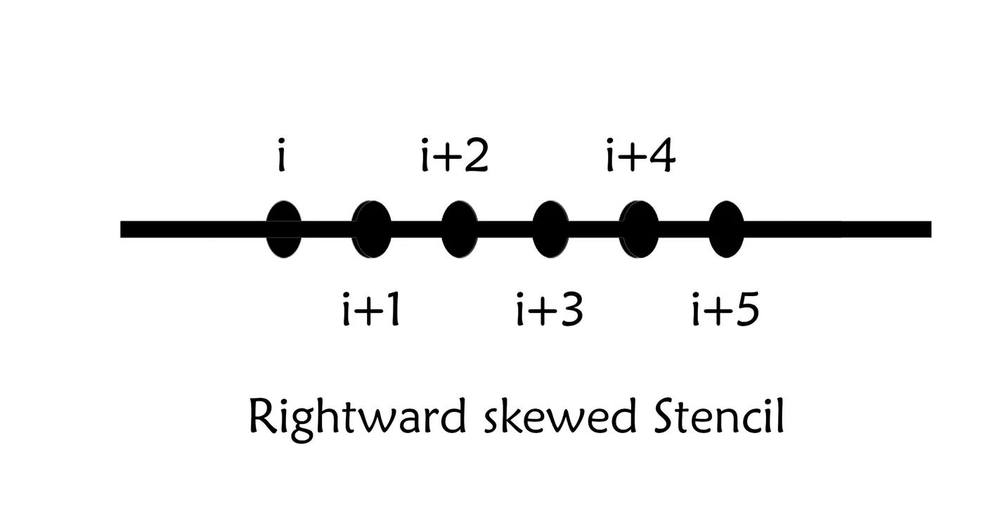
First, we assume that

`(d^2f)/(dx^2) = a*f(i) + b*f(i+1) + c*f(i+2) + d*f(i+3) + e*f(i+4) + g*f(i+5)`

Now our job is to find the values of a, b, c, d, e and g. for that we will be using the method of Taylors table.

	f(i)	f’(i) *ΔX	f’’(i) *ΔX2	f’’’(i) *ΔX3	f’’’’(i) *ΔX4	f’’’’’(i) *ΔX5
a * f(i)	a	0	0	0	0	0
b * f(i+1)	b	b	`b/2`	`b/6`	`b/24`	`b/120`
c * f(i+2)	c	2c	`(4*c)/2`	`(8*c)/6`	`(16*c)/24`	`(32*c)/120`
d * f(i+3)	d	3d	`(9*d)/2`	`(27*d)/6`	`(81*d)/24`	`(243*d)/120`
e * f(i+4)	e	4e	`(16*e)/2`	`(64*e)/6`	`(256*e)/24`	`(1024*e)/120`
g* f(i+5)	g	5g	`(25*g)/2`	`(125*g)/6`	`(625*g)/24`	`(3125*g)/120`
`(d^2f)/(dx^2)`	0	0	1	0	0	0

The above table will give a system of linear equation that is to be solved in order to find out the values of a, b, c, d, e. The system of equation can be represented as below.

a + b + c + d + e + g = 0
0a + b + 2c + 3d + 4e + 5g = 0
0a + b/2 + 2*c + 4.5*d + 8*e + 12.5*g = 1
0a + b/6 + (8*c)/6 + (27*d)/6 + (64*e)/6 + (125*g)/6 = 0
0a + b/24 + (16*c)/24 + (81*d)/24 + (256*e)/24 + (625*g)/24 = 0
0a + b/120 + (32*c)/120 + (243*d)/120 + (1024*e)/120 + (3125*g)/120 = 0

The above system of equations can be written in a matrix form AX= B

Where

`A = ((1,1,1,1,1,1),(0,1,2,3,4,5),(0,1/2,2,4.5,8,12.5),(0,1/6,8/6,27/6,64/6,125/6),(0,1/24,16/24,81/24,256/24,625/24),(0,1/120,32/120,243/120,1024/120,3125/120))`

`B = ((0),(0),(1),(0),(0),(0))` and

`X = ((a),(b),(c),(d),(e),(g))`

we will be getting values of a,b,c,d,e and g as 3.7500,-12.8333, 17.8333, -13.0000, 5.0833, and -0.8333 respectively.

if we are substituting values of this coefficient and making some arrangements we will be getting the scheme as

`(d^2f)/(dx^2) = ((15/4)* f(x) -(77/6)*f(x+Deltax) +(107/6)* f(x+2*Deltax) - 13 *f(x+3*Deltax) + (61/12)* f(x+4*Deltax) - (5/6)* f(x+5*Deltax))/((Deltax)^2)`

Determination of order of error.

To find the order of error first wee have to expand the complete Taylors table and then we have to substitute values of various coefficients. Then we will be getting an equation as follows.

`(d^2 f)/(dx^2) = f''(x) dx^2 + (0 + b + 64c + 729d + 4096e + 15625 g) f^(vi) dx^6/(6!) +HOT`

here HOT means Higher order terms

according to our auumption

`(d^2f)/(dx^2) = a*f(i) + b*f(i+1) + c*f(i+2) + d*f(i+3) + e*f(i+4) + g*f(i+5)`

`(a f(x) + b f(x+Deltax) + c f(x+2Deltax) + d f(x+3Deltax) + e f(x+4Deltax) + g f(x+5Deltax))/((Deltax)^2) = f''(x) + (0 + b + 64c + 729d + 4096e + 15625 g) f^(vi) (Deltax)^4/(6!) + HOT`

In this equation, power of the first terms contating `Deltax` is 4.so our scheme is of the order 4.

Lefttward skewed method

To obtain a fourth order truncation error we have to take 6 points (4+2) for a skewed case. All the points will be at the left side of the point of prime interest. The stencil representing the condition is shown below.

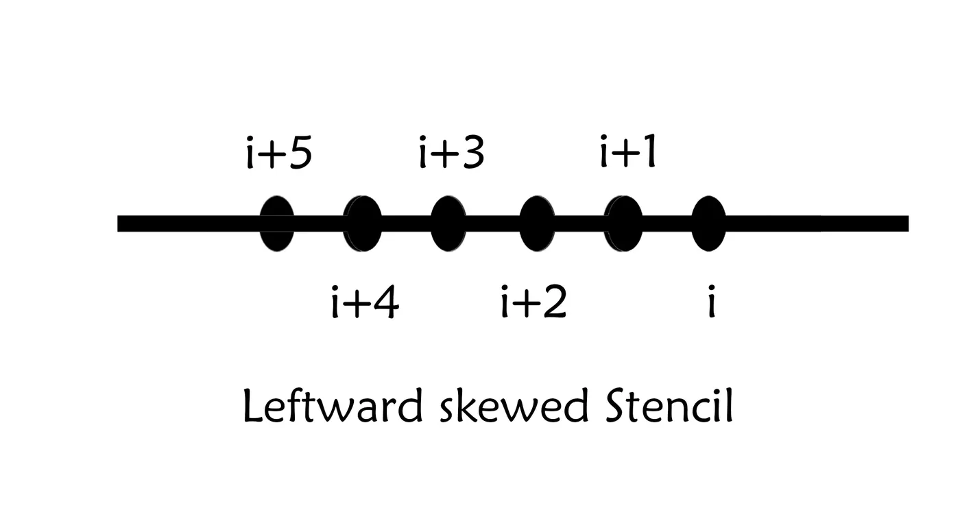
First, we assume that

`(d^2f)/(dx^2) = a*f(i) + b*f(i-1) + c*f(i-2) + d*f(i-3) + e*f(i-4) + g*f(i-5)`

Now our job is to find the values of a, b, c, d, e and g. for that we will be using the method of Taylors table.

	f(i)	f’(i) *ΔX	f’’(i) *ΔX2	f’’’(i) *ΔX3	f’’’’(i) *ΔX4	f’’’’’(i) *ΔX5
a * f(i)	a	0	0	0	0	0
b * f(i+1)	b	-b	`b/2`	`-b/6`	`b/24`	`-b/120`
c * f(i+2)	c	-2c	`(4*c)/2`	`(-8*c)/6`	`(16*c)/24`	`(-32*c)/120`
d * f(i+3)	d	-3d	`(9*d)/2`	`(-27*d)/6`	`(81*d)/24`	`(-243*d)/120`
e * f(i+4)	e	-4e	`(16*e)/2`	`(-64*e)/6`	`(256*e)/24`	`(-1024*e)/120`
g* f(i+5)	g	-5g	`(25*g)/2`	`(-125*g)/6`	`(625*g)/24`	`(-3125*g)/120`
`(d^2f)/(dx^2)`	0	0	1	0	0	0

The above table will give a system of linear equation that is to be solved in order to find out the values of a, b, c, d, e. The system of equation can be represented as below.

a + b + c + d + e + g = 0
0a - b - 2c - 3d - 4e - 5g = 0
0a + b/2 + 2*c + 4.5*d + 8*e + 12.5*g = 1
0a - b/6 - (8*c)/6 - (27*d)/6 - (64*e)/6 - (125*g)/6 = 0
0a + b/24 + (16*c)/24 + (81*d)/24 + (256*e)/24 + (625*g)/24 = 0
0a - b/120 - (32*c)/120 - (243*d)/120 - (1024*e)/120 - (3125*g)/120 = 0

The above system of equations can be written in a matrix form AX= B

Where

`A = ((1,1,1,1,1,1),(0,-1,-2,-3,-4,-5),(0,1/2,2,4.5,8,12.5),(0,-1/6,-8/6,-27/6,-64/6,-125/6),(0,1/24,16/24,81/24,256/24,625/24),(0,-1/120,-32/120,-243/120,-1024/120,-3125/120))`

`B = ((0),(0),(1),(0),(0),(0))` and

`X = ((a),(b),(c),(d),(e),(g))`

we will be getting values of a,b,c,d,e and g as 3.7500,-12.8333, 17.8333, -13.0000, 5.0833, and -0.8333 respectively.

if we are substituting values of this coefficient and making some arrangements we will be getting the scheme as

`(d^2f)/(dx^2) = ((15/4)* f(x) -(77/6)*f(x-Deltax) +(107/6)* f(x-2*Deltax) - 13 *f(x-3*Deltax) + (61/12)* f(x-4*Deltax) - (5/6)* f(x-5*Deltax))/((Deltax)^2)`

Determination of order of error.

To find the order of error first wee have to expand the complete Taylors table and then we have to substitute values of various coefficients. Then we will be getting an equation as follows.

`(d^2 f)/(dx^2) = f''(x) dx^2 + (0 + b + 64c + 729d + 4096e + 15625 g) f^(vi) dx^6/(6!) +HOT`

here HOT means Higher order terms

according to our auumption

`(d^2f)/(dx^2) = a*f(i) + b*f(i-1) + c*f(i-2) + d*f(i-3) + e*f(i-4) + g*f(i-5)`

`(a f(x) + b f(x-Deltax) + c f(x-2Deltax) + d f(x-3Deltax) + e f(x-4Deltax) + g f(x-5Deltax))/((Deltax)^2) = f''(x) + (0 + b + 64c + 729d + 4096e + 15625 g) f^(vi) (Deltax)^4/(6!) + HOT`

In this equation, power of the first terms contating `Deltax` is 4.so our scheme is of the order 4.

MATLAB FUNCTION

function [SKF,ERSKF,SKB,ERSKB,CEN,ERCEN] =taylersunafun(x,dx,analyticalderivative)
F=@(x)exp(x)*cos(x);


SKF = ((45*exp(x)*cos(x))+(-154*exp(x+dx)*cos(x+dx))+(214*exp(x+(2*dx))*cos(x+(2*dx)))+(-156*exp(x+(3*dx))*cos(x+(3*dx)))+(61*exp(x+(4*dx))*cos(x+(4*dx)))+(-10*exp(x+(5*dx))*cos(x+(5*dx))))./(12*(dx.^2));
ERSKF = abs(analyticalderivative - SKF);

SKB = ((45*exp(x)*cos(x))+(-154*exp(x-dx)*cos(x-dx))+(214*exp(x-(2*dx))*cos(x-(2*dx)))+(-156*exp(x-(3*dx))*cos(x-(3*dx)))+(61*exp(x-(4*dx))*cos(x-(4*dx)))+(-10*exp(x-(5*dx))*cos(x-(5*dx))))./(12*(dx.^2));
ERSKB = abs(analyticalderivative - SKB);

amid = -1/12;
bmid = 4/3;
cmid = -2.5000;
dmid = 4/3;
emid = -1/12;

CEN = ((-1*exp(x+(2*dx))*cos(x+(2*dx)))+(16*exp(x+dx)*cos(x+dx))+(-30*exp(x)*cos(x))+(16*exp(x-dx)*cos(x-dx))+(-1*exp(x-(2*dx))*cos(x-(2*dx))))./(12*(dx.^2));
ERCEN = abs(analyticalderivative - CEN);

end

MATLAB Main Program

clear all
close all
clc
%defining the function

x= pi;
dx= linspace(pi/400,pi/4,500)';

anayltical_derivative = -2*exp(x)*sin(x);

SKF = zeros(length(dx),1);
ERSKF = zeros(length(dx),1);
SKB = zeros(length(dx),1);
ERSKB = zeros(length(dx),1);
CEN = zeros(length(dx),1);
ERCEN = zeros(length(dx),1);
for i = 1:length(dx)
    [SKF(i),ERSKF(i),SKB(i),ERSKB(i),CEN(i),ERCEN(i)] = taylersunafun(x,dx(i),anayltical_derivative);
end

figure(1)
title('Error Comparison: 2nd derivative 4th order approximation with various schemes')
subplot(1,2,1)
loglog(dx,ERCEN)
hold on 
grid on
loglog(dx,ERSKF)
hold on
loglog(dx,ERSKB)
xlabel('log(dx)')
ylabel('log(error)')
legend('Central difference scheme','Forward difference scheme','Backward difference scheme','Location','best')


subplot(1,2,2)
plot(dx,ERCEN)
grid on
hold on 
plot(dx,ERSKF)
hold on
plot(dx,ERSKB)
xlabel('dx')
ylabel('error')
legend('Central difference scheme','Forward difference scheme','Backward difference scheme','Location','best')

Results

The proces of discritization has been done so that the second derivative of a function can be found out with a fourth order of truncation error. By using Taylor's table method Forward, Backward, and Central discritization has been done successfully. A MATLAB program is created to check the developed schemes.

The result obtained is shown below.

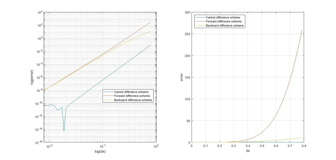
From the figure its clear that the error in central difference scheme is much smaller compared to the other schems. hence we will be employing the CDS where ever possible. but these schems can't be used at the boundary region because we won't be having preceding or succeeding points. The use of forward or backward difference scheme depends on the situation. If we have to find properties at downstream and we are having values at upstreame then we can use forward diffrence scheme, and if the case is reverse we have to stick on backward differencing scheme.

The zipped program file is attached below.