Steady state & Transient 2D Heat Conduction Analysis using MATLAB

Here We have to do analysis of transient as well as steady state heat conduction equation. The boundary conditions are given as Temperature at Top Boundary = 600 K, Temperature at Bottom Boundary = 900 K, Temperature at Left Boundary = 400 K and Temperature at Right Boundary = 800 K. and the error criteria is given as 1e-4. Here we will be assuming our lamina is of unit dimensions and grid spacing is uniform and equal in both directions. The number of nodes in both the directions are assumed to be 20 in both the cases. For the transient case we assume time starting from 0 and 2 seconds with a time step of 0.01 seconds.

Steady state conduction.

For a two-dimensional steady state heat conduction problem with no heat generation the governing equation will be as follows.

`(del^2T)/(delx^2)+(del^2T)/(dely^2)=0`

After discretization we will be getting expression for temperature distribution in the form of a FDE as shown below

`T(i,j) = (1/(kk))*(((T(i-1 , j)+T(i+1 , j))/(Deltax^2))+((T(i , j-1 ) + T(i , j+1 ))/(Deltay^2)))`

Here the term kk (kk is used because some times simply writing k may give a mis conception that it is thermal conductivity) is grid constant and is given by

`kk=2*((Deltax^2+Deltay^2)/(Deltax^2*Deltay^2))`

Here the PDE is converted in to system of algibraic equations. To solve this here I have used 3 methods. They are.

1 Jacobi’s method

The following equation is used in the jacobi's method.

`T(i,j) = (Told(i-1,j)+Told(i+1,j))/(kk*(Deltax^2)) + (Told(i,j-1)+Told(i,j+1))/(kk*(Deltay^2))`

Note that in Jacobi's method in a particular iteration we will be using values of previous iteration.

2 Gauss Seidel method

The following equation is used in the Gauss Seidel method.

`T(i,j)=(T(i-1,j)+T(i+1,j))/(kk*(Deltax^2)) + (T(i,j-1)+T(i,j+1))/(kk*(Deltay^2))`

Note that in Gauss Seidel method in a particular iteration we will be using latest values of variable, which may be from previous or current iteration.

3 Successive Over-Relaxation (SOR) method.

The following equation is used in the SOR method.

Here the first guss can be made by using either Gauss Sidel or Jacobi's method and then we have to applay SOR factor to get the actual value. Here I am using SOR with Gauss sidel meathod. the equations will be

`Tgs = (((T(i-1,j)+T(i+1,j))/dx^2) + ((T(i,j-1)+T(i,j+1))/dy^2))/(kk )`

and

`T(i,j)=(1-omega)*Told(i,j) + omega*(Tgs)`

here `omega` is SOR factor and optimum value of `omega` is given by

`omega_"optimum" = 2/(1+sin(pi*dx))`

MATLAB Code

Using the above concepts a MATLAB Code is made and is given below.

clear all
close all
clc

%Initializing the variables
nx = 20;
ny = nx;
x=linspace(0,1,nx);
y=linspace(0,1,ny);
dx =x (2)-x(1);
dy =y (2)-y(1);


kk = 2*((dx^2 + dy^2)/((dx^2) * (dy^2)));
tol = 1e-4;
T = 390*ones(ny,nx);

%boundary & initial Conditions
Ttop=600;
Tleft=400;
Tbottom=900;
Tright=800;
Tbottomright=0.5*(Tbottom+Tright);
Tbottomleft=0.5*(Tbottom+Tleft);
Ttopright=0.5*(Ttop+Tright);
Ttopleft=0.5*(Ttop+Tleft);

T(:,1)=Tleft;
T(:,nx)=Tright;
T(1,:)=Ttop;
T(ny,:)=Tbottom;
T(1,1)=Ttopleft;
T(ny,nx)=Tbottomright;
T(1,nx)=Ttopright;
T(ny,1)=Tbottomleft;
[X, Y] = meshgrid(x,y);
Tinitial=T;

for solver = 1:3
            % Jacobi method == solver1
            % Gauss seidel method == solver2
            % Successive over relaxation method == solver3
    if solver==1
    [Tjack,errorjack,jac_iter,solution_timejac] = jackfun(tol,T,dx,dy,nx,ny,kk);
    T=Tinitial;
    
    figure(1)
    plott = contourf(X,Y,Tjack,'edgecolor','none');
    set(gca,'YDIR','reverse');
    colormap(jet);
    title(sprintf('Solution of 2D steady state heat conduction using Jacobi method \n No of Iterations: %d',jac_iter));
    xlabel('X')
    ylabel('Y')
    saveas(gca,'2D steady heat conduction Jacobi method method.png')
    
    display('~~~~~~~~~~~~~~~~~~~~~~~~~~~~~~~~~~~~~~~~~~~~~');
    display('2D steady heat conduction jacobi method');
    display('~~~~~~~~~~~~~~~~~~~~~~~~~~~~~~~~~~~~~~~~~~~~~');
    fprintf('No of iteration taken in jacobi method is %d \n',jac_iter);
    fprintf('Time taken for Jacobi Method is %d \n',solution_timejac);
    fprintf('Error in Jacobi Method is %d \n',errorjack);
    
elseif solver==2
    [TGS,errorGS,GS_iter,solution_timegs] = GSfun(tol,T,dx,dy,nx,ny,kk);
    T=Tinitial;
    
    figure(2)
    plotu = contourf(X,Y,TGS,'edgecolor','none');
    set(gca,'YDIR','reverse');
    colormap(jet);
    title(sprintf('Solution of 2D steady state heat conduction using Gauss Sidel method \n No of Iterations: %d',GS_iter));
    xlabel('X')
    ylabel('Y')
    saveas(gca,'2D steady heat conduction Gauss Sidel method method.png')

    display('~~~~~~~~~~~~~~~~~~~~~~~~~~~~~~~~~~~~~~~~~~~~~');
    display('2D steady heat conduction Gauss sidel method');
    display('~~~~~~~~~~~~~~~~~~~~~~~~~~~~~~~~~~~~~~~~~~~~~');
    fprintf('No of iteration taken in Gauss sidel method is %d \n',GS_iter);
    fprintf('Time taken for Gauss sidel method is %d \n',solution_timegs);
    fprintf('Error in Gauss sidel Method is %d \n ',errorGS);

elseif solver==3
    [TSOR,errorSOR,sor_iter,solution_timeSOR,Omega] = sorfun(tol,T,dx,dy,nx,ny,kk);
    figure(3);
    plotv = contourf(X,Y,TSOR,'edgecolor','none');
    set(gca,'YDIR','reverse');
    colormap(jet);
    title(sprintf('Solution of 2D steady state heat conduction using SOR method \n No of Iterations: %d',sor_iter));
    xlabel('X')
    ylabel('Y')
    saveas(gca,'2D steady heat conduction SOR method method.png')
    
    display('~~~~~~~~~~~~~~~~~~~~~~~~~~~~~~~~~~~~~~~~~~~~~');
    display('2D steady heat conduction SOR method');
    display('~~~~~~~~~~~~~~~~~~~~~~~~~~~~~~~~~~~~~~~~~~~~~');
    fprintf('Omega value used in SOR method is %d \n',Omega);
    fprintf('No of iteration taken in SOR method is %d \n',sor_iter);
    fprintf('Time taken for SOR method is %d \n',solution_timeSOR);
    fprintf('Error in SOR Method is %d \n ',errorSOR);
    end
end

MATLAB Functions

For Computiong the results with 3 functons three MATLAB Functions are created. and are given below

1. Function for Jacobi's Method (jackfun.m)

function [Tjack,error,jac_iter,solution_time] = jackfun(tol,T,dx,dy,nx,ny,kk)
jac_iter=0;
Told=T;
error = 1;
tic;
while(error)>tol
    for i = 2:nx-1
        for j = 2:ny-1
                term1=(Told(i-1,j)+Told(i+1,j))/(kk*(dx^2));
                term2=(Told(i,j-1)+Told(i,j+1))/(kk*(dy^2));
                T(i,j)=term1+term2;
        end
    end
        error=max(max(abs(T-Told)));
        Told=T;        
        jac_iter =jac_iter+1;
end
solution_time=toc;
Tjack = T;
end

2. Function for Gauss-Sidel Method (GSfun.m)

function [TGS,error,GS_iter,solution_time] = GSfun(tol,T,dx,dy,nx,ny,kk)
GS_iter=0;
Told=T;
error = 1;
tic;
while(error)>tol
    for i = 2:nx-1
        for j = 2:ny-1
                term1=(T(i-1,j)+T(i+1,j))/(kk*(dx^2));
                term2=(T(i,j-1)+T(i,j+1))/(kk*(dy^2));
                T(i,j)=term1+term2;
        end
    end
        error=max(max(abs(T-Told)));
        Told=T;        
        GS_iter =GS_iter+1;
end
solution_time=toc;
TGS = T;
end

3. Function for SOR Method (sorfun.m)

function [TSOR,error,sor_iter,solution_time,OMEGA] = sorfun(tol,T,dx,dy,nx,ny,kk)

%terms used in the equation
OMEGA=2/(1+sin(pi*dx));
error = 1;
sor_iter=0;
Told=T;

tic
while(error>tol) %convergence_loop
     for i =2:nx-1
          for j =2:ny-1
               Tgs = (((T(i-1,j)+T(i+1,j))/dx^2) + ((T(i,j-1)+T(i,j+1))/dy^2))/kk ;
               T(i,j)=(1-OMEGA)*Told(i,j) + OMEGA*(Tgs);
          end
     end
     error = max(max(abs(T-Told)));
     Told=T; %updating old values
     sor_iter=sor_iter+1;
     
   
end
solution_time=toc;
TSOR = T;
end

Command window Output

~~~~~~~~~~~~~~~~~~~~~~~~~~~~~~~~~~~~~~~~~~~~~
2D steady heat conduction jacobi method
~~~~~~~~~~~~~~~~~~~~~~~~~~~~~~~~~~~~~~~~~~~~~
No of iteration taken in jacobi method is 805 
Time taken for Jacobi Method is 1.367340e-02 
Error in Jacobi Method is 9.987319e-05 
~~~~~~~~~~~~~~~~~~~~~~~~~~~~~~~~~~~~~~~~~~~~~
2D steady heat conduction Gauss sidel method
~~~~~~~~~~~~~~~~~~~~~~~~~~~~~~~~~~~~~~~~~~~~~
No of iteration taken in Gauss sidel method is 432 
Time taken for Gauss sidel method is 7.818100e-03 
Error in Gauss sidel Method is 9.865272e-05 
 ~~~~~~~~~~~~~~~~~~~~~~~~~~~~~~~~~~~~~~~~~~~~~
2D steady heat conduction SOR method
~~~~~~~~~~~~~~~~~~~~~~~~~~~~~~~~~~~~~~~~~~~~~
Omega value used in SOR method is 1.717336e+00 
No of iteration taken in SOR method is 60 
Time taken for SOR method is 6.822400e-03 
Error in SOR Method is 8.376349e-05

Results of Steady State Heat Conduction Analysis

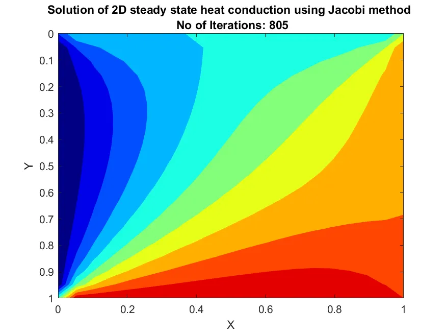
Temperature Contour obtained from Jacobi's Method is given below.

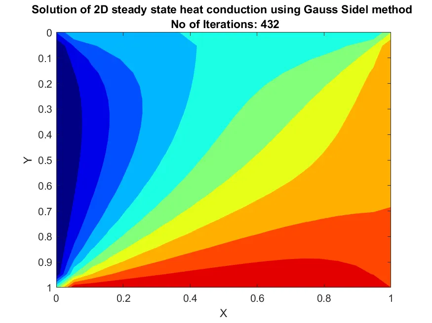
Temperature Contour obtained from Gauss-Sidel Method is given below.

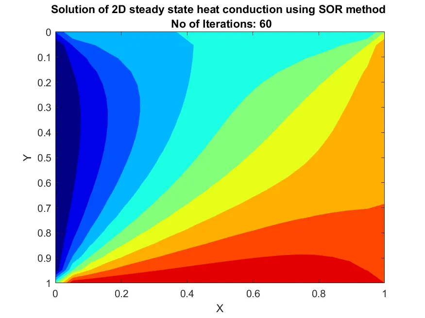
Temperature Contour obtained from SOR Method is given below.

Transient Conduction

For a two-dimensional transient conduction problem with no heat generation the governing equation will be as follows.

`(del^2T)/(delx^2)+(del^2T)/(dely^2)=1/alpha*(delT)/(delt)`

where `alpha` is thermal diffusivity.

After discretization we will be getting expression for temperature distribution in the form of a FDE as shown below

`T(i,j)=Told(i,j)+k1*(Told(i-1,j)-(2*Told(i,j))+Told(i+1,j))+k2*(Told(i,j-1)-(2*Told(i,j))+Told(i,j+1))`

where

`k1=alpha((Deltat)/(Deltax^2))` and

`k2=alpha((Deltat)/(Deltay^2))`

Here the PDE is converted in to system of algibraic equations. To solve this here I have used 6 methods. They are. These methods can be classified brody into 2 sections. implicit and explicit. in explicit method while calculating value for a particular time steps we will be using values from previous timesteps only. in implicit methods we will be using values from the current timesteps. The six methods are given below

1 Jacobi's explicit method

2 Gauss seidel explicit method

3 Successive over relaxation explicit method

4 Jacobi's Implicit method

5 Gauss seidel Implicit method

6 Successive over relaxation Implicit method

MATLAB Code

Using the above concepts a MATLAB Code is made and is given below.

%2D heat conduction-transient analysis

clc
clear all
close all

%grid points

nx=20;
ny=nx;
x=linspace(0,1,nx);
y=linspace(0,1,ny);
[X, Y] = meshgrid(x,y);
dx=x(2)-x(1);
dy=y(2)-y(1);

start_time=0;
end_time=2;
dt=0.01;
t= [start_time:dt:end_time];
    T = 300*ones(ny,nx);
    % Boundary conditions
    %boundary & initial Conditions
    Ttop=600;
    Tleft=400;
    Tbottom=900;
    Tright=800;
    Tbottomright=0.5*(Tbottom+Tright);
    Tbottomleft=0.5*(Tbottom+Tleft);
    Ttopright=0.5*(Ttop+Tright);
    Ttopleft=0.5*(Ttop+Tleft);

    T(:,1)=Tleft;
    T(:,nx)=Tright;
    T(1,:)=Ttop;
    T(ny,:)=Tbottom;
    T(1,1)=Ttopleft;
    T(ny,nx)=Tbottomright;
    T(1,nx)=Ttopright;
    T(ny,1)=Tbottomleft;
    Tinitial = T;

    tolerance=1e-4;
    alpha=0.05;
    k1=(alpha*dt)/(dx^2);
    k2=(alpha*dt)/(dy^2);

for solverNumber = 1:6
    % Explicit 
        % Jacobi method == solver1
        % Gauss seidel method == solver2
        % Successive over relaxation method == solver3
        % Implicit
        % Jacobi method ==solver4
        % Gauss seidel method ==solver5
        % Successive over relaxation method ==solver6
        
        T=Tinitial;
    
    % Solver method used
        solver=solverNumber;
        
        %Explicit

    %Jacobi method
    if solver==1
        [TjackE,jac_iterE,solving_timeJE,errorJE] = Jacobi_explicit_trans(t,nx,ny,tolerance,T,k1,k2);

            %plot
            figure(1)
            C = contourf(X,Y,TjackE,'edgecolor','none');
            set(gca,'YDIR','reverse');
            colormap(jet);
            clabel(C,'FontSize',12);
            title(sprintf('Solving transient state heat conductionn using Jacobi-explicit solver \n No of Iterations: %d',jac_iterE));
            xlabel('X')
            ylabel('Y')
            saveas(gca,'2D transient heat conduction jac-explicit method.png')


            % Iteration and Time display
            display('****************************************************************');
            display('2D heat conduction solved using Jacobi-explicit method');
            display('****************************************************************');
            fprintf('No of iteration taken is %d \n ',jac_iterE);
            fprintf('Time taken for solving is %f  \n',solving_timeJE);
            fprintf('The error obtained is %f \n',errorJE);



    %Gauss Seidel Method
    elseif solver==2

        [TGSE,GS_iter,solving_timeGSE,errorGSE] = Gs_explicit_trans(t,nx,ny,tolerance,T,k1,k2);
        %plot

        figure(2)
        C = contourf(X,Y,TGSE,'edgecolor','none');
        set(gca,'YDIR','reverse');
        colormap(jet);
        clabel(C,'FontSize',12);
        title(sprintf('Solving transient state heat conductionn using Gauss Seidel-explicit solver \n No of Iterations: %d',GS_iter));
        xlabel('X')
        ylabel('Y')
        saveas(gca,'2D transient heat conduction GS-explicit method.png')

        % Iteration and Time display
        display('****************************************************************');
        display('2D heat conduction solved using Gauss Seidel-explicit method');
        display('****************************************************************');
        fprintf('No of iteration taken is %d \n',GS_iter);
        fprintf('Time taken for solving is %f \n',solving_timeGSE);
        fprintf('The error obtained is %f \n',errorGSE);

    %Successive Over Relaxation Method
    elseif solver==3
        [TSORE,SORE_iter,solving_timeSORE,errorSORE] = SOR_explicit_Trans(t,nx,ny,tolerance,T,k1,k2,dx);

            %plot
            figure(3)
            C = contourf(X,Y,TSORE,'edgecolor','none');
            set(gca,'YDIR','reverse');
            colormap(jet);
            clabel(C,'FontSize',12);
            title(sprintf('Solving transient state heat conductionn using SOR-explicit solver \n No of Iterations: %d',SORE_iter));
            xlabel('X')
            ylabel('Y')
            saveas(gca,'2D transient heat conduction SOR-explicit method.png')

            % Iteration and Time display
            display('*******************************************************');
            display('2D heat conduction solved using Successive over relaxation-explicit method');
            display('*******************************************************');
            fprintf('No of iteration taken is %d \n',SORE_iter);
            fprintf('Time taken for solving is %f \n',solving_timeSORE);
            fprintf('The error obtained is %f \n',errorSORE);


    %Implicit

    %Jacobi method
    elseif solver==4
        [TJacI,JacI_iter,solving_timeJackI,errorJacI] = Jacobi_implicit_trans(t,nx,ny,tolerance,T,k1,k2);

        %plot
        figure(4)
        C = contourf(X,Y,TJacI,'edgecolor','none');
        set(gca,'YDIR','reverse');
        colormap(jet);
        clabel(C,'FontSize',12);
        title(sprintf('Solving transient state heat conductionn using Jacobi-implicit solver \n No of Iterations: %d',JacI_iter));
        xlabel('X')
        ylabel('Y')
        saveas(gca,'2D transient heat conduction jac-implicit method.png')

        % Iteration and Time display
        display('****************************************************************');
        display('2D heat conduction solved using Jacobi-implicit method');
        display('****************************************************************');
        fprintf('No of iteration taken is %d \n ',JacI_iter);
        fprintf('Time taken for solving is %f \n',solving_timeJackI);
        fprintf('The error obtained is %f \n',errorJacI);


    %Gauss Seidel method
    elseif solver==5
        [TGSI,GSI_iter,solving_timeGSI,errorGSI] = Gs_implicit_trans(t,nx,ny,tolerance,T,k1,k2);

            %plot
            figure(5)
            C = contourf(X,Y,TGSI,'edgecolor','none');
            set(gca,'YDIR','reverse');
            colormap(jet);
            clabel(C,'FontSize',12);
            title(sprintf('Solving transient state heat conductionn using GS-implicit solver \n No of Iterations: %d',GSI_iter));
            xlabel('X')
            ylabel('Y')
            saveas(gca,'2D transient heat conduction GS-implicit method.png')


            % Iteration and Time display
            display('****************************************************************');
            display('2D heat conduction solved using Gauss Seidel-Implicit method');
            display('****************************************************************');
            fprintf('No of iteration taken is %d \n',GSI_iter);
            fprintf('Time taken for solving is %f \n',solving_timeGSI);
            fprintf('The error obtained is %f \n',errorGSI);    


    %Successive Over Relaxation Method
    elseif solver==6
        [TSORI,SORI_iter,solving_timeSORI,errorSORI] = SOR_implicit_trans(t,nx,ny,tolerance,T,k1,k2,dx);

            %Plotting 
            figure(6)
            C = contourf(X,Y,TSORI,'edgecolor','none');
            set(gca,'YDIR','reverse');
            colormap(jet);
            clabel(C,'FontSize',12);
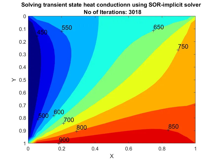
            title(sprintf('Solving transient state heat conductionn using SOR-implicit solver \n No of Iterations: %d',SORI_iter));
            xlabel('X')
            ylabel('Y')
            saveas(gca,'2D transient heat conduction SOR-implicit method.png')

            % Iteration and Time display
            display('*******************************************************');
            display('2D heat conduction solved using SOR-Implicit method');
            display('*******************************************************');
            fprintf('No of iteration taken is %d \n',SORI_iter);
            fprintf('Time taken for solving is %f \n',solving_timeSORI);
            fprintf('The error obtained is %f \n',errorSORI);
    end 
        
        
end

MATLAB Functions

For Computiong the results with 3 functons three MATLAB Functions are created. and are given below.

1 Jacobi's explicit method (Jacobi_explicit_trans.m)

%Jacobi-Explicit method

function [Tjack,jac_iter,solving_time,error] = Jacobi_explicit_trans(t,nx,ny,tolerance,T,k1,k2)
jac_iter=0;
Told=T;
tic
% Time loop
for k=1:length(t)
    error=9e9;
    % Convergence loop
    while (error>tolerance)
    % Nodal loop
        for i=2:nx-1
         for j=2:ny-1
            T(i,j)=Told(i,j)+k1*(Told(i-1,j)-(2*Told(i,j))+Told(i+1,j))+k2*(Told(i,j-1)-(2*Told(i,j))+Told(i,j+1));  
         end
        end
            error=max(max(abs(T-Told)));
            Told=T; %updating old values
            jac_iter=jac_iter+1;
    end
end
solving_time=toc;
Tjack=T;
end

2 Gauss seidel explicit method (Gs_explicit_trans.m)

%Gauss Seidel-Explicit method
function [TGS,gs_iter,solving_time,error] = Gs_explicit_trans(t,nx,ny,tolerance,T,k1,k2)
gs_iter=0;
Told=T;
error=9e9;
tic
%time loop
for k=1:length(t)
    %Convergence loop
    while (error>tolerance)
        %nodal loop
        for i=2:nx-1
            for j=2:ny-1
                T(i,j)=Told(i,j)+k1*(T(i-1,j)-(2*Told(i,j))+Told(i+1,j))+k2*(T(i,j-1)-(2*Told(i,j))+Told(i,j+1));
            end
        end

        error=max(max(abs(T-Told)));
        Told=T;
        gs_iter=gs_iter+1;
    end
end
solving_time=toc;
TGS=T;
end

3 Successive over relaxation explicit method (SOR_explicit_Trans.m)

%Successive over relaxation-Explicit method

function [TSORE,sor_iter,solving_timeSORE,errorSORE] = SOR_explicit_Trans(t,nx,ny,tolerance,T,k1,k2,dx)
Omega=2/(1+sin(pi*dx)); % relaxation factor
sor_iter=0;
Told=T;
errorSORE=9e9;
tic
%Time loop
for k=1:length(t)
    % Convergence loop
    while (errorSORE>tolerance)
        %nodal loop
        for i=2:nx-1
            for j=2:ny-1
                 T(i,j)= Omega*(Told(i,j)+k1*(T(i-1,j)-(2*Told(i,j))+Told(i+1,j))+k2*(T(i,j-1)-(2*Told(i,j))+Told(i,j+1)))+((1-Omega)*Told(i,j));    
            end
        end    
        errorSORE=max(max(abs(T-Told)));
        Told=T; %updating old values
        sor_iter=sor_iter+1;
    end
end
solving_timeSORE=toc;
TSORE = T;
end

4 Jacobi's Implicit method (Jacobi_implicit_trans.m)

%Jacobi-Implicit method

function [TJacI,jac_iter,solving_time,error] = Jacobi_implicit_trans(t,nx,ny,tolerance,T,k1,k2);

jac_iter=0;
Told=T;
T_prev_dt=T;
term1=(1+(2*k1)+(2*k2))^-1;
term2=k1*term1;
term3=k2*term1;

tic
%time loop
for k=1:length(t)
    error=9e9;
    
    %convergence loop
    while (error>tolerance)
        
    %nodal loop
        for i=2:nx-1
         for j=2:ny-1
                H=(Told(i-1,j)+Told(i+1,j));
                V=(Told(i,j-1)+Told(i,j+1));
                T(i,j)=(T_prev_dt(i,j)*term1)+(term2*H)+(term3*V);
    
         end
        end  
        
      error=max(max(abs(T-Told)));
      Told=T; %updating old values
      jac_iter=jac_iter+1;

    end
    
    T_prev_dt=T; % updating previous time step values
    
end

solving_time=toc;

TJacI = T;

end

5 Gauss seidel Implicit method (Gs_implicit_trans.m)

%Gauss Seidel-Implicit method

function [TGSI,gs_iter,solving_time,error] = Gs_implicit_trans(t,nx,ny,tolerance,T,k1,k2)

gs_iter=0;
Told=T;
T_prev_dt=T;
term1=(1+(2*k1)+(2*k2))^-1;
term2=k1*term1;
term3=k2*term1;

tic
%time loop
for k=1:length(t)
    error=9e9;
    
    %convergence loop
    while (error>tolerance)
        
    %nodal loop
        for i=2:nx-1
         for j=2:ny-1
                H=(T(i-1,j)+Told(i+1,j));
                V=(T(i,j-1)+Told(i,j+1));
                T(i,j)=(T_prev_dt(i,j)*term1)+(term2*H)+(term3*V);
    
         end
        end  
        
      error=max(max(abs(T-Told)));
      Told=T;
      gs_iter=gs_iter+1;

    end
    
T_prev_dt=T;% Updating previous time step values

end

solving_time=toc;
TGSI =T;


end

6 Successive over relaxation Implicit method (Gs_explicit_trans.m)

%Successive over relaxation-Implicit method

function [TSORI,sor_iter,solving_time,error] = SOR_implicit_trans(t,nx,ny,tolerance,T,k1,k2,dx)


sor_iter=0;
Told=T;
T_prev_dt=T;
term1=(1+(2*k1)+(2*k2))^-1;
term2=k1*term1;
term3=k2*term1;
Omega=2/(1+sin(pi*dx)); %relaxation factor

tic
%time loop
for k=1:length(t)
    error=9e9;
    
    %convergence loop
    while (error>tolerance)
        
    %nodal loop
        for i=2:nx-1
         for j=2:ny-1
                H=(T(i-1,j)+Told(i+1,j));
                V=(T(i,j-1)+Told(i,j+1));
                T(i,j)=Omega*((T_prev_dt(i,j)*term1)+(term2*H)+(term3*V))+(1-Omega)*(T_prev_dt(i,j));    
         end
        end  
      error=max(max(abs(T-Told)));
      Told=T; % update old values
      sor_iter=sor_iter+1;

    end
    
T_prev_dt=T; %Update previous time step value

end
solving_time=toc;
TSORI = T;
end

Command window Output

****************************************************************
2D heat conduction solved using Jacobi-explicit method
****************************************************************
No of iteration taken is 1312 
 Time taken for solving is 0.039392  
The error obtained is 0.000014 
****************************************************************
2D heat conduction solved using Gauss Seidel-explicit method
****************************************************************
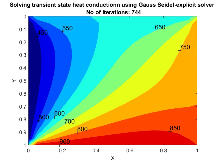
No of iteration taken is 744 
Time taken for solving is 0.019900 
The error obtained is 0.000100 
*******************************************************
2D heat conduction solved using Successive over relaxation-explicit method
*******************************************************
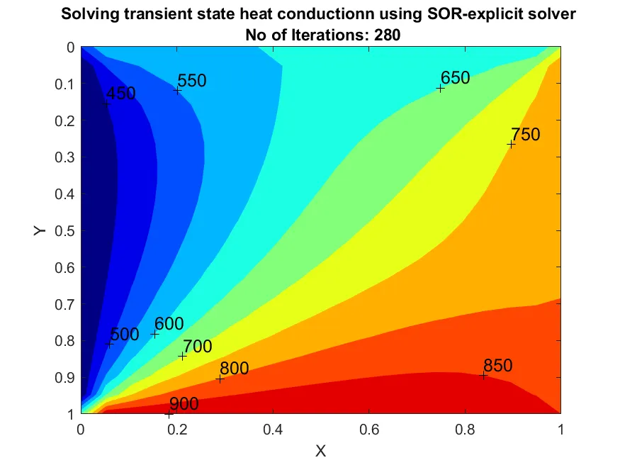
No of iteration taken is 280 
Time taken for solving is 0.008358 
The error obtained is 0.000099 
****************************************************************
2D heat conduction solved using Jacobi-implicit method
****************************************************************
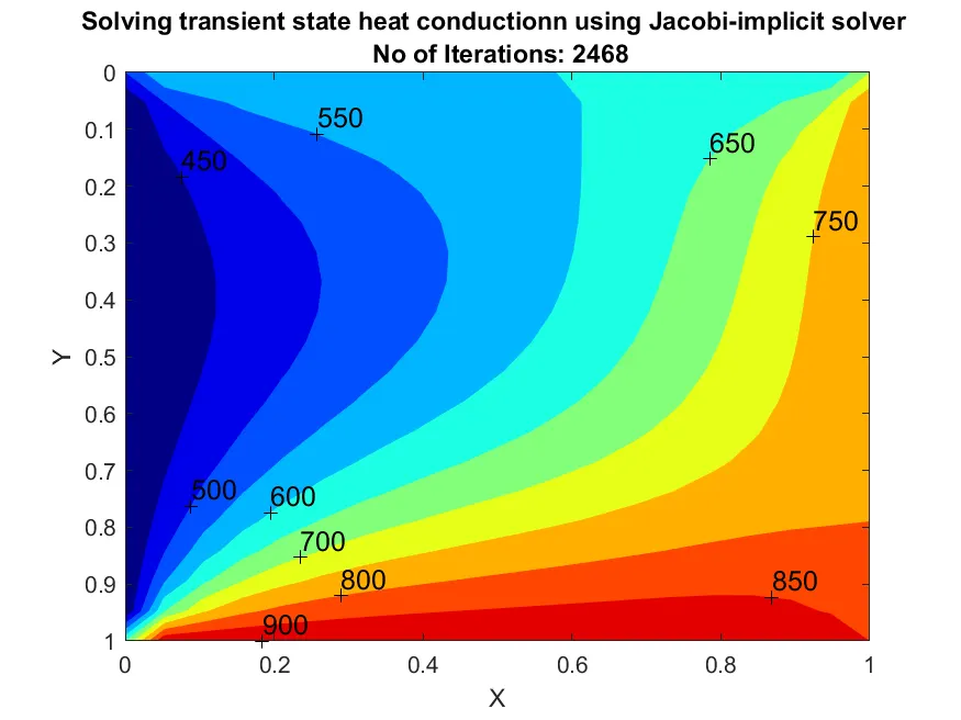
No of iteration taken is 2468 
 Time taken for solving is 0.051714 
The error obtained is 0.000071 
****************************************************************
2D heat conduction solved using Gauss Seidel-Implicit method
****************************************************************
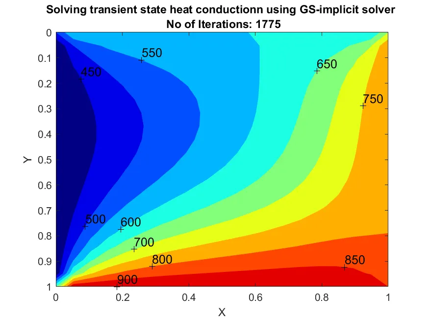
No of iteration taken is 1775 
Time taken for solving is 0.028633 
The error obtained is 0.000053 
*******************************************************
2D heat conduction solved using SOR-Implicit method
*******************************************************
No of iteration taken is 3018 
Time taken for solving is 0.064689 
The error obtained is 0.000082 

Results of Transient Heat Conduction Analysis

Temperature Contour obtained from Jacobi's explicit Method is given below.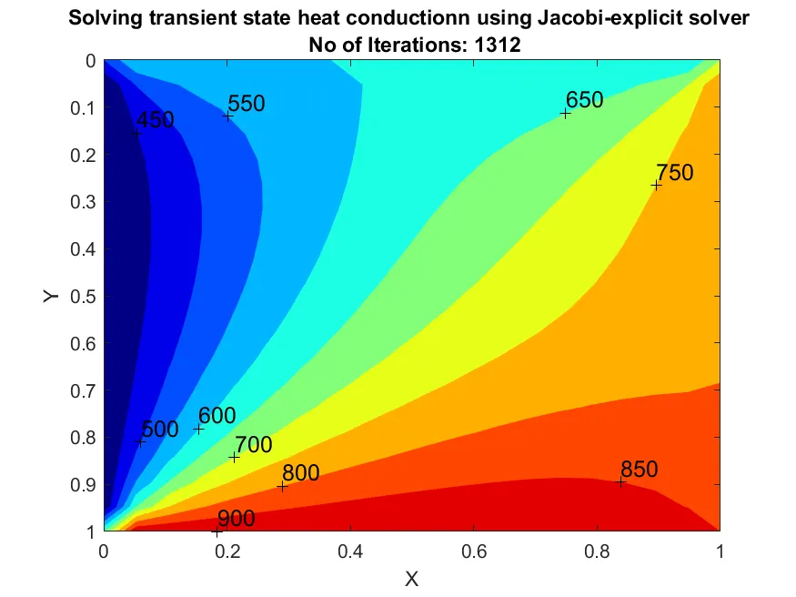

Temperature Contour obtained from Gauss-Sidel explicit Method is given below.

Temperature Contour obtained from SOR explicit Method is given below.

Temperature Contour obtained from Jacobi's implicit Method is given below.

Temperature Contour obtained from Gauss Sidel implicit Method is given below.

Temperature Contour obtained from SOR implicit Method is given below.

Conclusion

Transient and steady state analysis of heat conduction in a unit squre lamina hving uniform and equal grid spacing has been done with various methods and results has been obtained. The Temparature distribution is obtained and plotted using all the methods.

In the case of steady heat conduction the number of iteration taken for converging the solution by various methods adopted is given below.

Number of iteration taken in jacobi method is 805

Number of iteration taken in Gauss sidel method is 432

Number of iteration taken in SOR method is 60

the higher number of iteration for jacobi's method (almost double compared to Gauss sidel method) says that Number of iterations can be reduced if we are using updated values during an iterative procedure.
By using an appropriate value of SOR we have reduced the number of iteration by a factor of 7.2 for gauss sidel method and this indicates a good property of SOR. From this we can say that adopting SOR method is a good scheme for steady state conduction as of now.

In the case of steady heat conduction the error prsent in the solution in the various methods adopted is given below.

Error in Jacobi Method is 9.987319e-05

Error in Gauss sidel Method is 9.865272e-05

Error in SOR Method is 8.376349e-05

From these values we can infer that SOR method will be giving minimum error along with a minimum number of iteration and its really appreciated. SOR methods will be providing around 1.178 times less error compared to Gauss sidel method.

Since the error is higher for Jacobi's methos we can say that updating the values during the iterative process will decrese the error and the convergence will be faster.

In the case of steady heat conduction the Time taken for convergence for various methods adopted is given below.

Time taken for Jacobi Method is 1.136790e-02

Time taken for Gauss sidel method is 1.127080e-02

Time taken for SOR method is 4.103900e-03

From the first sight itsel we can go for SOR method since the order of magnitude of time taken itself varries for SOR method. The SOR method is giving solution with minimum error, minimum time and minimum number of iteration and hence its the ideal one we can depend up on. It gives around 2.75 times faster response compared to Gauss sidel method.

Since the time taken is higher for Jacobi's methos we can say that updating the values during the iterative process will decrese the time required and the convergence will be faster.

In the case of Transient heat conduction the number of iteration taken for converging the solution by various methods adopted is given below.

While looking in to the Command window out put for Transient conduction we can say that for explicit schemes the trend si similar to steady state heat conduction as discussed above. but when coming to the implicit scheme the trend reverses. So some optimizations in algorithams is needed for transient solutions.

I am attaching the codes below as a compressed .RAR file below.