Finite Volume Method (FVM)

One important feature of finite volume schemes is their conservation properties. Since they are based on applying conservation principles over each small control volume, global conservation is also ensured. The method starts by dividing the flow domain into a number of small control volumes as shown below.

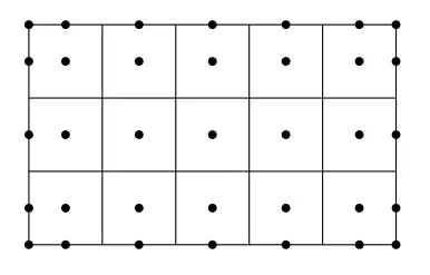
For the sake of simplicity here we have considerd rectangular grids with equal grid spacing but its not mandatory. The grid points where variables are stored are typically defined as being at the centre of each control volume. Extra boundary nodes are often added, as shown in the figure to applay boundary conditions. The transport equation(s) are then integrated over each control volume.

As an example lets consider 1D steady state heat condution without heat generation as an example.

The governng equation is

`d/(dx)(k* (dT)/(dx)) = 0`

Consider 1D heat conduction through a long bar having constant Area A of cross section and isotropic in nature. we will be dividing block through n control volume as shown below.

Here we will be first dealing with interior control volumes and then will take care of boundary control volumes.

Consider an arbitrary control volume i

so our conservation equation says heat comming into the control volume = heat going out of the control voumume.

which implies that

`kA*(T_i-T_(i-1))/(delx) = kA*(T_(i+1)-T_i)/(delx)`

which on re arrangement can be written in the following form.

`a_i T_i = a_(i-1) T_(i-1) + a_(i+1) T_(i+1)`

where

`a_(i-1) = (k*A)/(delx)`

`a_(i+1) = (k*A)/(delx)`

`a_i = a_(i-1) + a_(i+1)`

Applying a Constant temperature boundary condition for control volume one's left face will give following results.

`kA*(T_A-T_(1))/((delx)/2) = kA*(T_(2)-T_1)/(delx)`

which on re arrangement can be written as

`a_1 T_1 = a_0 T_0 + a_2 T_2 + Su`

where

`a_0 = 0`

`a_(2) = (k*A)/(delx)`

`a_1 = a_0 + a_2 - S_p`

`S_p = - (2*kA)/(delx)`

`S_u = (2*kA)/(delx) T_A`

Applying a Constant temperature boundary condition for control volume n's right face will give following results.

`kA*(T_(n-1)-T_(n))/(delx) = kA*(T_(n)-T_(B))/((delx)/2)`

which on re arrangement can be written as

`a_n T_n = a_(n-1) T_(n-1) + a_(n+1) T_(n+1) + Su`

where

`a_(n+1) = 0`

`a_(n-1) = (k*A)/(delx)`

`a_n = a_(n-1) + a_(n+1) - S_p`

`S_p = - (2*kA)/(delx)`

`S_u = (2*kA)/(delx) T_B`

These will be giving a system of simultanious equation with n equations and n variables. it can be solved by using Gaus sidel method. This is how a problem is woked out using FVM.

FDM vs FVM

FDM is based on the differential form of governing equation where as FVM is based on integral form of the equation. Since the FDM is developed based on differntial form it can't handle discontinuities where as FVM is capable of the same. Between a differential and an integral scheme (integral scheme scores in terms of error). Differential schemes are faster and error can be minimized if you have regular grids (squares and rectangles). Integral schemes are slightly slower but score over FDM when the mesh is irregular. Using variable transformation method gives an approx solution of property but is very much time consuming and complex. Most of the commercial software like FLUENT (FVM) are either FVM or FEM.

Interpolation schemes

Interpolation schems are used inorder to find value of a field variable of interest at a point which is not coinciding with any particular node. Through discritized equation we will be only having solution for the field variable at discrete points to give a continuous variation and a rough approximation of variable at intermediate location we will be depending up on interpolation schemes. In FVM the major interpolation schemes are Upwind Interpolation Scheme (UDS), Linear Interpolation Scheme, Quadratic Upwind Interpolation Scheme, Hybrid Interpolation Scheme, Total variation Diminishing Scheme and some other Schemes like PRESTO, MUSCL etc...

1. Upwind Interpolation Scheme (UDS)

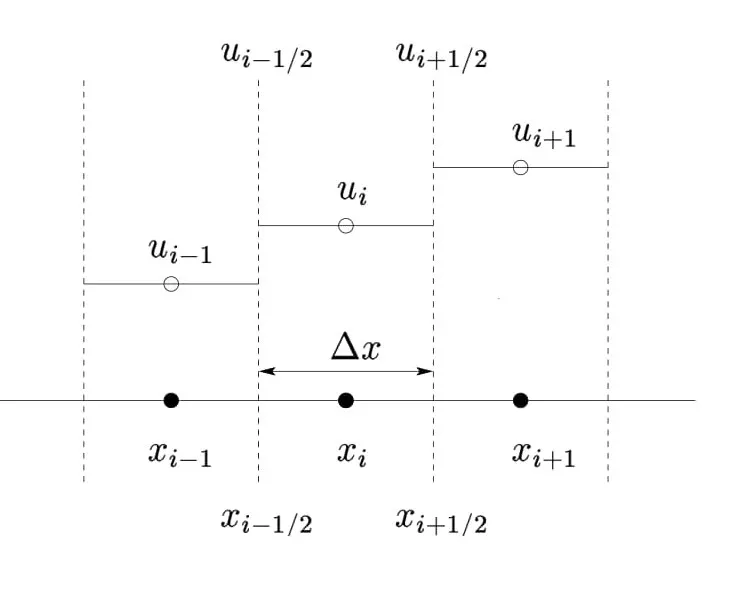
The upwind interpolation scheme (UDS) for approximating the value of a variable f at the east face of a control volume is given by

`f_e= {(f_(p ) if (v.n)_e>0),(f_E if (v.n)_e<0):}`

It is generally used convection dominated problems (i.e pe >1).

The values of the interface is given by:

for v > 0, we have

`u_(i-1/2) approx u_(i-1) , u_(i+1/2) approx u_(i)`

`I_c approx v {u_i - u_(i-1)}/{Deltax}`- Backward difference

for v < 0, we have

`u_(i-1/2) approx u_(i) , u_(i+1/2) approx u_(i+1)`

`I_c approx v {u_(i+1) - u_i}/{Deltax}` - Forward difference

Taylor series expansion

`vu_(i+1/2) = vu_i - {vDeltax}/2({delu}/{delx})_(i+1/2) - v(Deltax)^2/8({del^2u}/{delx^2})_(i+1/2) +.....`

a first order accurate flux approximation, the leading truncation error resembles a diffusive flux `d{delu}/{delx}` with `d = {vDeltax}/2` being numerical diffusion coefficient.

2. Linear Interpolation Scheme

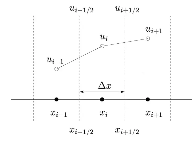
To approximate the values of variables at CV face centre by linear interpolation of the values at two nearest computational nodes. This is equivalent to the use of the central difference scheme of first order derivative, and hence it is also known as central difference scheme. This also leads to very simple approximation of evaluation of gradients required for evaluation of diffusive fluxes. The relation is given as follows:

`f_e = f_E lambda_e + f_p(1-lambda_e)` where `lambda_e = {x_e - x_p}/{x_E-x_p}`

Interpolation polynomial:

`p_1(x) = u_L.{x_R-x}/{x_R-x_L} + u_R.{x-x_L}/{x_R-x_L}`

Average interface values are given by,

`u_(i-1/2) approx {u_(i-1) + u_i}/2`and `u_(i+1/2) approx {u_(i) + u_(i+1)}/2`

`I_c approx v.{u_(i+1) - u_(i-1)}/{2.Deltax}` - Central differencing

Taylor series approximation

`u_(i+1) = u_(i+1/2) + {Deltax}/2 .({delu}/{delx})_(i+1/2) +(Deltax)^2/8.({del^2u}/{delx^2})_(i+1/2) + .....`

`u_i = u_(i+1/2) - {Deltax}/2 .({delu}/{delx})_(i+1/2) +(Deltax)^2/8.({del^2u}/{delx^2})_(i+1/2) + .....`

From the above expression we get,

`u_(i+1/2) = {u_i + u_(i+1)}/2 - (Deltax)^2/8.({del^2u}/{delx^2})_(i+1/2)+...`

The approximation is second order accurate. It is the simplest and most widely used interpolation for evaluation of gradients reqired for evaluation of diffusive fluxes.

3. Quadratic Upwind Interpolation Scheme

This approximates the value of variable at CV face centre by quadratic interpolation of the values at three nearest computational nodes (one downstream node, D and two upstream nodes, U). It is third order accurate for both uniform and nonuniform grids.

`f_e = f_U + g_1(f_D - f_U) + g_2(f_(UU) -f_u)`

`g_1 = {(x_e - x_U)(x_e - x_(UU))}/{(x_D - x_U)(x_D-x_(UU))`

`g_2 = {(x_e - x_U)(x_e - x_D)}/{(x_(UU) - x_D)(x_(UU)-x_(U))`

The relation obtained as:

`phi_e = 6/8phi_c + 3/8phi_D - 1/8phi_(UU)`

4. Hybrid Interpolation Scheme

It is the blend of CDS and UDS scheme, based on Peclet number

`f_e = gammaf_(CDS) + (1-gamma)f_(UDS)`

5. Total variation Diminishing Scheme

`f_e = f_p + 1/2 psi(r)(f_E - f_p)`

where `psi` is the flux limiter.

Flux Limiters

The Flux limiters or slope limiters are used inorder to provide the stability and accuaracy in a flow field incase if there is a presence of discontinuity like shock waves. The flux limiter functions will take values varrying from 0 to 1. If the location of point is near to discontinuity it will take value equal to zero and as it moves away from the dis continuity it's value will approch 1. The concepts of flux limiters emenates from an intersting behaviour of neumerical scheme and its accuaracy. Numerical approximation using higher order spatial discretization schemes results in better accuracy but exhibits spurious oscillations near discontinuities such as shocks. On the other hand, lower order spatial discretization schemes remain stable near discontinuities but dampen out the distributions because of their dissipative nature. Hence in order to capture discontinuities, high resolution schemes are desired - which are highly accurate and stable throughout the domain. by introducing the flux limiter function we will be considering both the schemes and will be taking a weighted avarage method. Hence it switches between higher order scheme and lower order scheme for numerical representation of flux, thereby keeping the scheme stable and accurate throughout the flow doamin.

consider 1D- semi-discrete scheme

`(du_i)/(dt)+1/(Deltax_i)[F(u_(i+1/2)) - F(u_(i-1/2))] = 0`

`F(u_(i+1/2)) & F(u_(i-1/2))` these are edge fluxes for the ith cell

`F(u_(i+1/2)) = f_(i+1/2)^(low) - phi(ri)(f_(i+1/2)^(low)-f_(i+1/2)^(high))`

`F(u_(i-1/2)) = f_(i-1/2)^(low) - phi(ri)(f_(i-1/2)^(low)-f_(i-1/2)^(high))`

`f^(high)` - low precision , high resolution flux

`f^(low)`- high precidion , low resolution flux

`phi(r)`- flux limiter function

`r_i = (u_i-u_(i-1))/(u_(i+1)-u_i)`

'r' reperesents the ratio of successive gradients on the solution mesh.

`phi(r)ge 0`

this is the limiter function case

if limiter function = 0 , then there will be a low resolution and sharp gradient.

if limiter function > 0 , then there will be a high resolution and +ve gradient.