Week 5 - Rayleigh Taylor Instability

RAYLEIGH TAYLOR INSTABILITY

OBJECTIVES:

1. Some practical CFD models have been based on the mathematical analysis of Rayleigh Taylor waves. And also explain how these mathematical models have been adapted for CFD calculations.
2. Perform the Rayleigh Taylor instability simulation for 2 different mesh sizes with the base mesh being 0.5 mm. Compare the results by showing the animations.
3. Explain why a steady-state approach might not be suitable for these types of simulations.
4. Run one more simulation with water and user-defined material(density = 400 kg/m³, viscosity = 0.001 kg/m-s) for refined mesh.
5. Define the Atwood Number. Find out the Atwood number for both cases and explain how the variation in the Atwood number in the above two cases affects the behavior of the instability.

THEORY:

Rayleigh Taylor Instability (RTI):

• Rayleigh observed that if two fluids (i.e lighter and heavier fluid) when were mixed together such that the denser fluid is on top of the lighter fluid, due to the gravity and the density variation the interface of the liquid is not stable.
• This instability of the interface between the different densities of fluid when the lighter fluid is accelerated towards the heavier fluid is knowns as Rayleigh-Taylor Instability.
• It is a dynamic process where the system tries to reduce its combined potential energy.

CFD models based on mathematical analysis of Rayleigh Taylor waves:

Mass diffusion model:

• The mass diffusion equation describes the transport of mass and energy due to model viscosity and hence drives actual mixing in the fluids.
• Even if any configuration is Rayleigh-Taylor unstable, the diffusion process could be responsible for significant mixing if the viscosity is sufficiently large.

Single fluid model:

1) Potential flow model

• This model is valid for all instability changes from the very linear stage through the early non-linear but limited to the Atwood number of 1.
• In this model, the single mode perturbation expands, the flow equation to second order around the bubble tips, hence obtaining an ordinary differential equation for the bubble velocity.

2) Buoyancy drag model

• It is valid for every Atwood number but limited to non-linear stages of the instability.
• It uses ordinary differential equations to evolve the width of the mixing layer. The bubble, spikes, or amplitudes are described by balancing the inertia, buoyancy, and drag forces.
• This model cannot deal with multiple mixing interfaces; cannot be easily extended to two or three dimensions, and as a rule, does not address demixing, also known as counter gradient transport i.e. reduction of total fluid masses within the mixing zone.
• To address the above problems, multifluid models have to be used.

3) Besnard-Harlow-Rauenzahn(BHR)

• It is a more advanced version of the single-fluid model.
• The BHR model is based on the evolution equations arising from second-order correlations and gradient-diffusion approximations.
• Using a mass-weighted-averaged decomposition, the original BHR model includes the full transport equation for Reynold's stresses, turbulent mass-flux velocity, density fluctuations, and turbulent kinetic energy dissipation rate.

Multi-Fluid model:

1) Two equation K-L turbulence model

• The K-L turbulence model involves the equation for turbulent kinetic energy (K) and turbulent length scale (L).
• The starting point for deriving the model equations is the buoyancy-drag models for the self-similar growth for RT instabilities.

2) Three-equation K-L-a turbulence model

• The three-equation model was developed as an extension of the two-equation K-L model by including a third equation for the turbulent mass-flux velocity.

3) Four-equation K-L-a-b turbulence model

• The four-equation model was developed as an extension of three equation K-L-a model by including a fourth equation for density-specific volume covariance.
• The model can accurately reflect the effect of changes in density fluctuations.

SIMULATION PROCEDURE:

Step 1: Geometry (SpaceClaim)

• Geometry is created with two different components air and water on top of each other.
• The dimensions of the constraint domain are 20 x 20 mm for each surface. Both surfaces are equal in dimension.

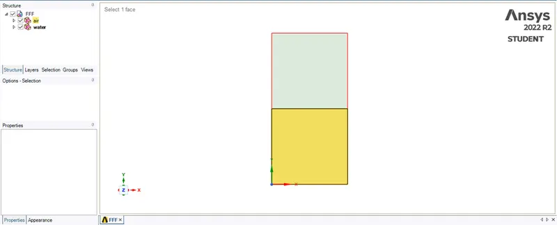
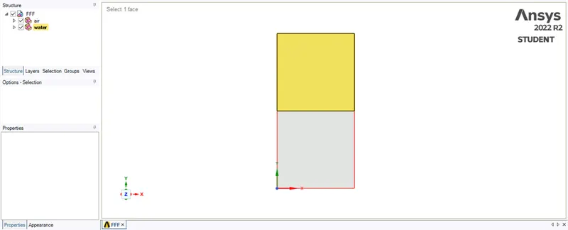
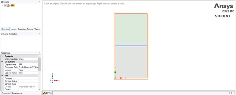
• The interface between the surface is shared using the sharePrep tool to share information through the interface and to get a conformal mesh.

Step 2: Mesh (Meshing)

• Case 1- Baseline mesh: element size = 0.5mm

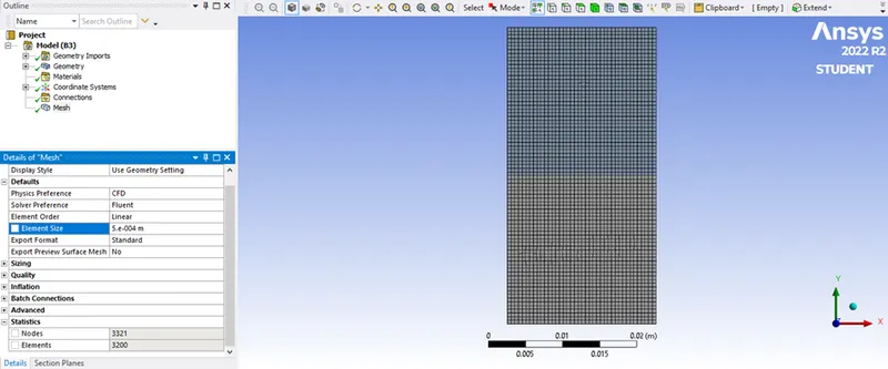
• Case 2- Refined mesh: element size = 0.2mm

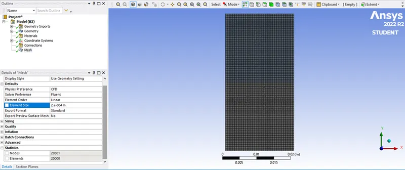
• Case 3- Refined mesh(with user defined fluid): element size = 0.2mm

Step 3: Setup and Solution (Fluent)

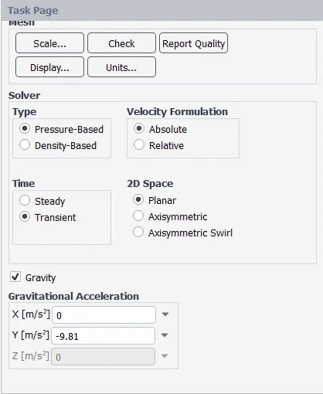
• A transient state simulation is performed using Pressure Based solver with Gravity enabled,

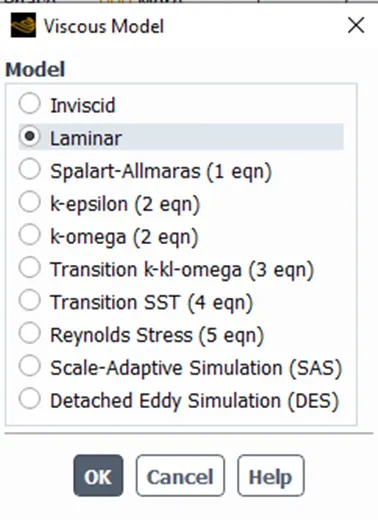
• The Laminar model is preferred as the velocity is low,

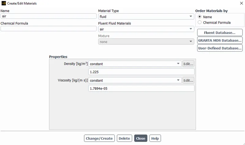
• The three materials to be used are added from the fluent database and the user-defined fluid is added manually,

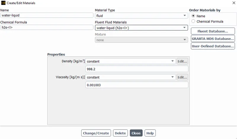
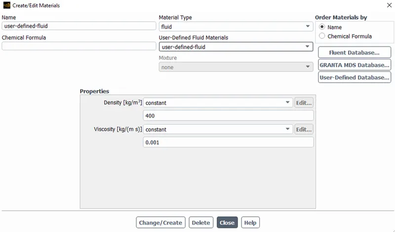
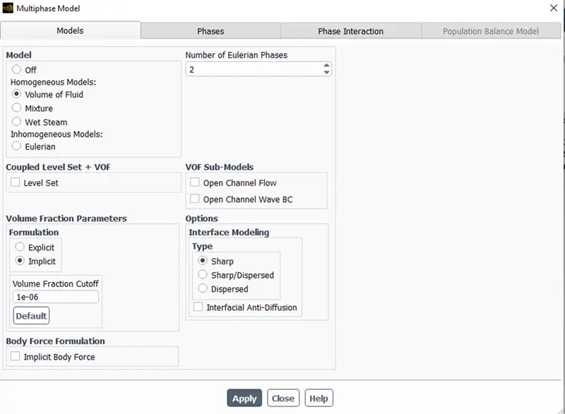
• The multiphase model is used with implicit formulation,

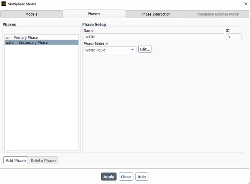
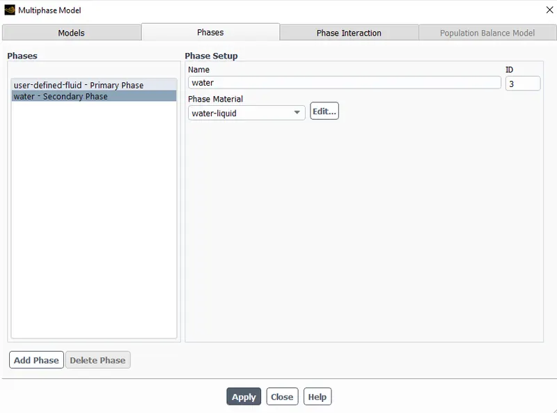
• The phases are named as follow for case 1 and 2,

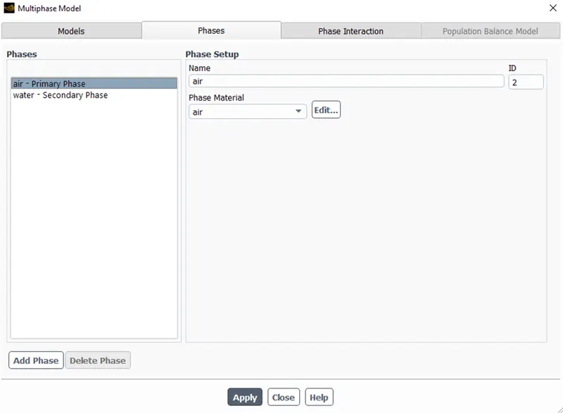
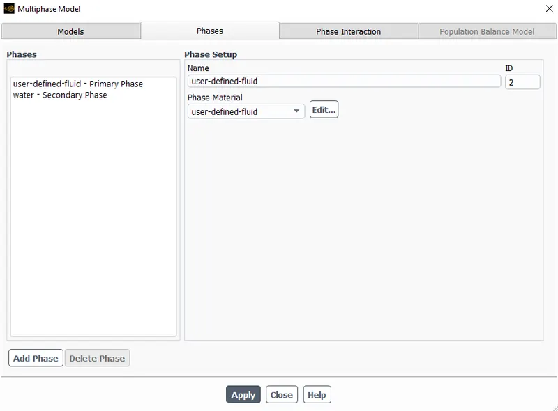
• For case 3,

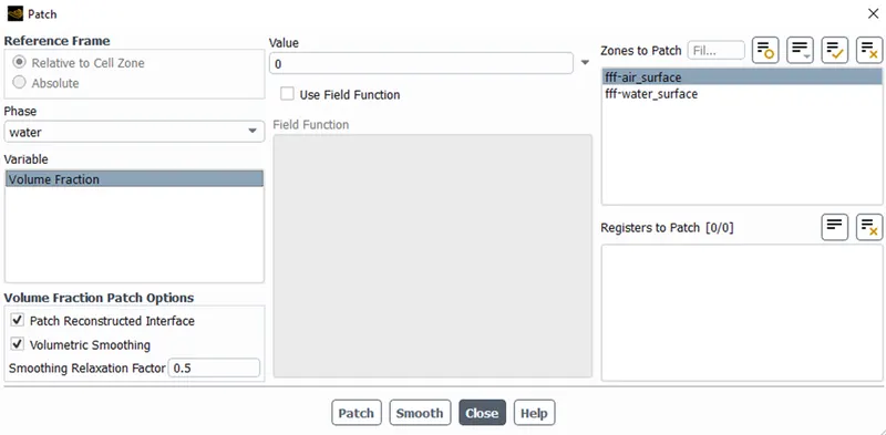
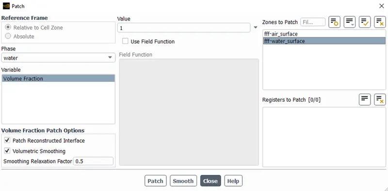
• The standard initialization is done to enable contour creation and patching.
• The water is patched such that `alpha` = 0 at the air surface and 1 at the water surface,

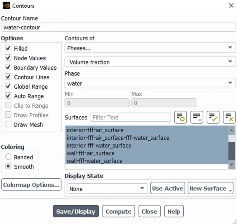
• The contour is created for phases at all surfaces,

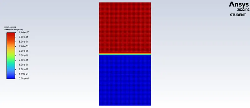
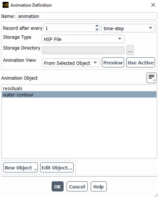
• The Solution animation is created for the phase contour,

• The solution is calculated for the three different cases.

OUTPUTS:

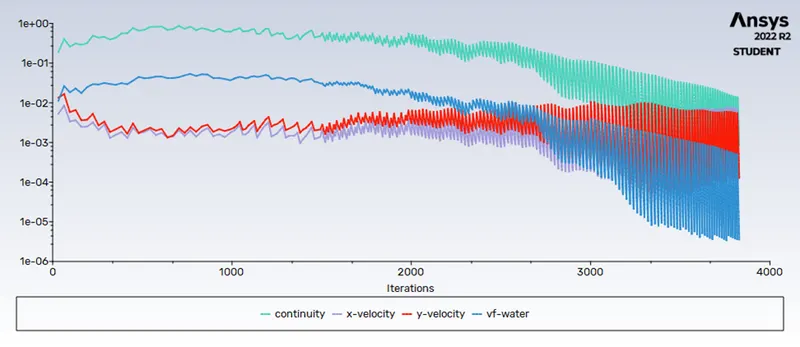
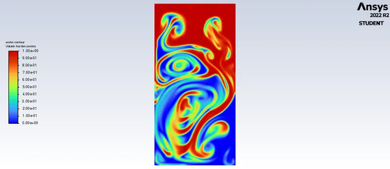
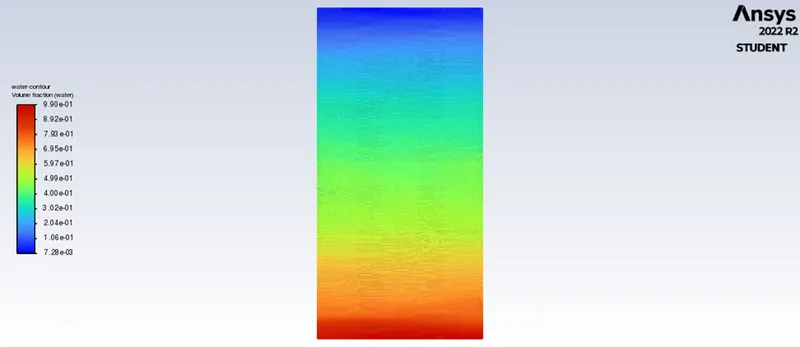
Residual plots with some sample frames:

1) Case 1- Baseline mesh:

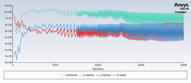
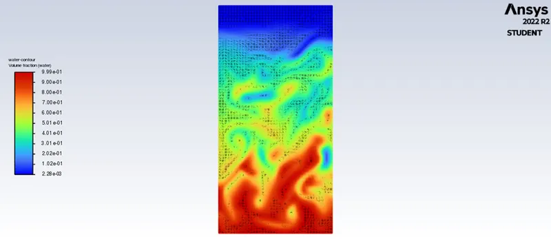
2) Case 2- Refined mesh:

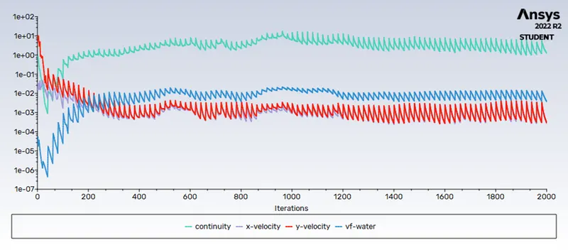
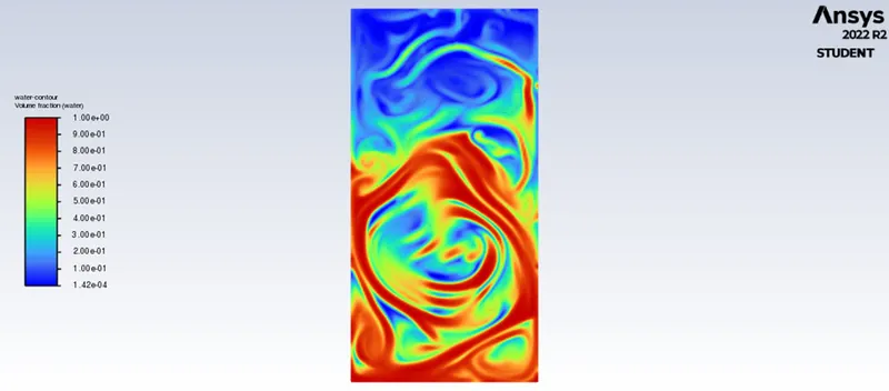
3) Case 3- Refined mesh(with user-defined fluid):

Animations:

1) Case 1- Baseline mesh:

https://drive.google.com/file/d/1EqxoNEVaXnCvwjI_tX8tRB4V3IC1EG7_/view?usp=sharing

2) Case 2- Refined mesh:

https://drive.google.com/file/d/1HsE9Q774FxbkQ5SD32lwHagBONB3MCpe/view?usp=sharing

3) Case 3- Refined mesh(with user-defined fluid):

https://drive.google.com/file/d/1FYWCx_DEF0F0QqD6dTMVx-LjWNL9oHks/view?usp=sharing

OBSERVATION:

Why a steady-state approach might not be suitable for these types of simulations?

• From the above results, we can observe the instabilities that we are trying to capture are changing unpredictably as a function of time.
• The steady-state approach is not time-dependent (doesn't capture the timesteps) and only solves the end result.
• The transient approach is preferred over the steady-state approach.

Atwood Number:

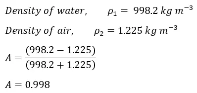
• It is a dimensionless number that is used to study hydrodynamic instabilities in density-stratified flows.

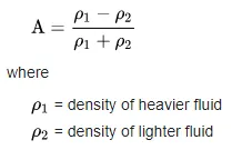
• The Atwood Number for cases 1 and 2:

• The Atwood Number for case 3:

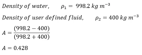
• Atwood number is an important parameter in the study of Rayleigh-Taylor instability.
• For an Atwood number close to 0, Rayleigh Taylor instability flows take the form of symmetric “fingers” of fluid. This was observed in case 3.
• For an Atwood number close to 1, the much lighter fluid below the heavier fluid takes the form of larger bubble-like plumes which was observed in cases 1 and 2.

The effect of mesh size on simulation:

• The finer mesh captured the instability better than the baseline mesh.
• But refining had an impact on the computational time as it increased drastically.
• If we want to study the instability of the interface at every timestep clearly then mesh refinement is recommended.

CONCLUSION:

• CFD models based on the mathematical analysis of Rayleigh Taylor waves were explained.
• Rayleigh Taylor instability simulation was performed successfully for 3 different cases and outputs were verified for using the Atwood number.