Week 5 - Rayleigh Taylor Instability

                                         REPORT ON REYLEIGH TAYLOR INSTABILITY

AIM 

1. To Perform the Rayleigh Taylor instability simulation for 2 different mesh sizes with the base mesh being 0.5 mm. Compare the results by showing the animations( Attach them from your google drive). Observe the differences in the animation and explain the effect of mesh size on simulation. Also, explain why a steady-state approach might not be suitable for these types of simulation.[ Choose Air and Water for this simulation]
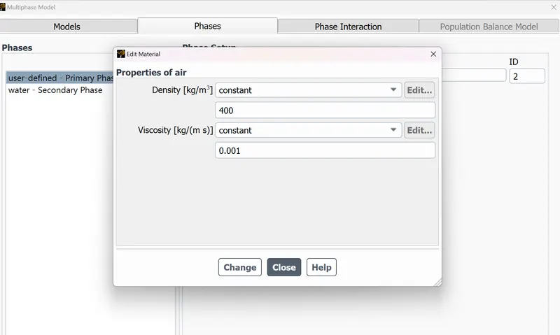
2. Run one more simulation with water and user-defined material(density = 400 kg/m³, viscosity = 0.001 kg/m-s) for refined mesh. 
3. What are some practical CFD models that have been based on the mathematical analysis of Rayleigh Taylor waves? In your own words, explain how these mathematical models have been adapted for CFD calculations.
4. Define the Atwood Number. Find out the Atwood number for both the cases and explain how the variation in Atwood number in the above two cases affects the behavior of the instability. 

THEORY

Practical CFD models that have been based on  the mathematical analysis of Rayleigh Taylor waves also explaining how these mathematical models have been adapted for CFD calculations.

Rayleigh Taylor Model - The Rayleigh–Taylor instability, or RT instability, is an Instability of an interface between two Fluids of different densities which occurs when the lighter fluid is pushing the heavier fluid. In this instability the denser fluid placed on the top mixes with the lighter fluid due to the presence of gravity. This results in the development of bubbles in the mixing area.

One example we can say is the mixing of water and kerosene or oil, where the two liquids does not mix with each other because of the difference in their densities and while mixing we can see the formation of bubbles. This is noted by Reighleigh and Taylor resulted in naming the process as instability and later it is known to be Reighleigh-Taylor instability.Examples include the behaviour of water suspended above oil in the gravity of Earth, mushroom clouds like those from volcanic eruptions and atmospheric nuclear explosions, supernova explosions in which expanding core gas is accelerated into denser shell gas, instabilities in plasma fusion reactors and inertial confinement fusion.

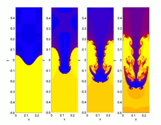
In the above image we can see the instability that is created due to the mixing of two immiscible fluids.

Practical CFD models that have been based on mathematical analysis of RT waves

1. Kelvin-Helmholtz instability
2. Richtmyer-Meshkov instability
3. Plateau-Rayleigh instability

 Kelvin-Helmholtz instability:

This instability typically occurs when there is velocity shear in a single continuous fluid, or additionally where there is a velocity difference across the interface between two fluids. A common example is seen when wind blows across a water surface, the instability constant is able to manifest itself through waves on water surface. The Kelvin-Helmholtz instability is not only restricted to a water surface as clouds, but is evident through other natural phenomena as ocean and the sun's corona. The theory predicts the onset of instability and transition to turbulent flow in fluids of different densities moving at various speeds. This instability occurs where there is a velocity shear or velocity difference between the interface of the two fluids.

Richtmyer-Meshkov instability:

Occurs when two fluids of different density are impulsively accelerated.Normally this is by the passage of a Shock wave.The development of the instability begins with small amplitude perturbations which initially grow linearly with time.This is followed by a nonlinear regime with bubbles appearing in the case of a light fluid penetrating a heavy fluid, and with spikes appearing in the case of a heavy fluid penetrating a light fluid.A chaotic regime eventually is reached and the two fluids mix.This instability can be considered the impulsive-acceleration limit of the Rayleigh Taylor Instability.

Example

Supersonic combustion in a Scramjet may benefit from RMI as the fuel-oxidants interface is enhanced by the breakup of the fuel into finer droplets. 

Plateau-Rayleigh instability

 This instability, often just called the Rayleigh instability, explains why and how a falling stream of fluid breaks up into smaller packets with the same volume but less surface area. It is related to the RTI and is part of a greater branch of fluid dynamics concerned with fluid thread breakup. This fluid instability is exploited in the design of a particular type of ink jet technology whereby a jet of liquid is perturbed into a steady stream of droplets. The driving force of the Plateau–Rayleigh instability is that liquids, by virtue of their surface tension, tend to minimize their surface area. It is part of a greater branch of fluid dynamics concerned with fluid - thread Breakup

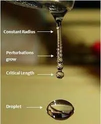
Example : Water dripping from tap changes its shape into spherical due to this instability.In other words the formation of small droplets when water is dripping from a faucet/tap. When a segment of water begins to separate from the faucet, a neck is formed and then stretched. If the diameter of the faucet is big enough, the neck doesn't get sucked back in, and it undergoes a Plateau–Rayleigh instability and collapses into a small droplet.

Inkjet Printing: Continuous ink jet printers (as opposed to drop-on-demand ink jet printers) generate a cylindrical stream of ink that breaks up into droplets prior to staining printer paper. By adjusting the size of the droplets using tunable temperature or pressure perturbations and imparting electrical charge to the ink, inkjet printers then steer the stream of droplets using electrostatics to form specific patterns on printer paper

PROCEDURE

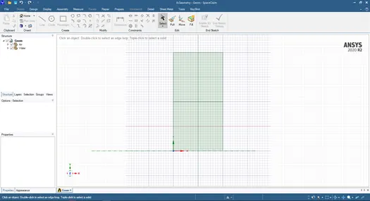
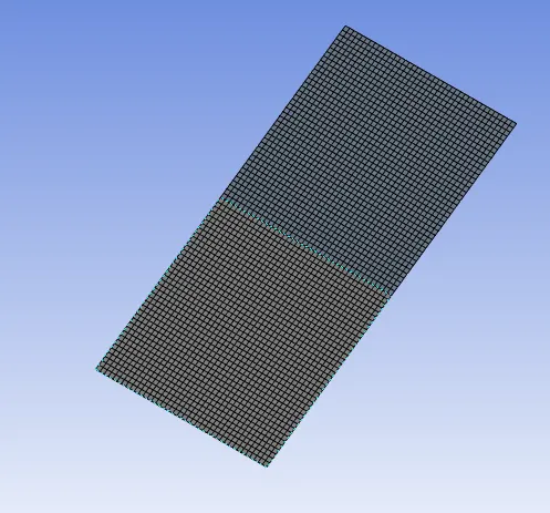
The first step is creating the geometry. We create two 2D square box one top of the other, which we assume 20cm each side and the upper box has the denser fluid and the walls are shared using share topology.

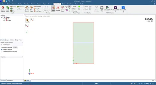
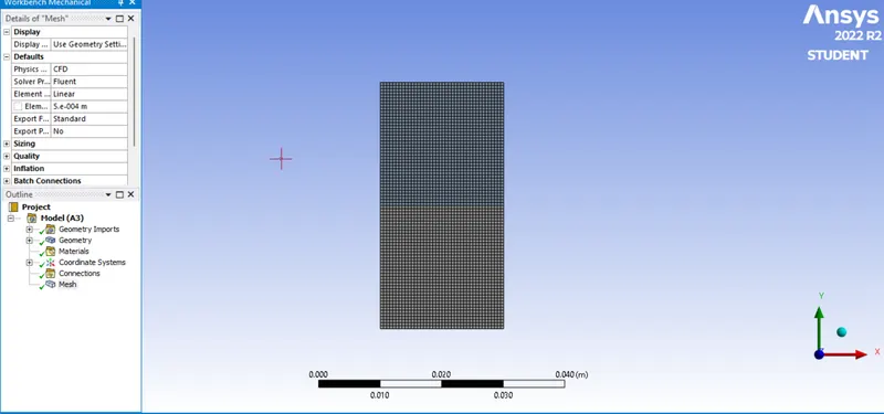
Then we create the mesh first we start with the base line mesh with mesh size of 0.5 mm

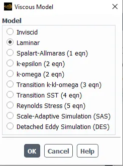
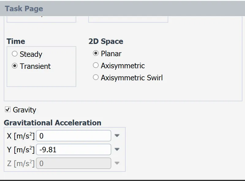
Then we set up the physics where we use transient state model as we are supposed to find the instability as a function of time. Also we use the pressure based solver because the flow is laminar and the density is constant. Also we use the volume of fluid method which is used to find out the position of interface between the two immiscible fluids

We add gravity in the set up because it helps in the downward motion of the water and mixing it with the air present in the lower box.

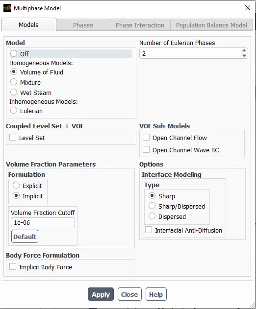
Then we add the multiphase where, primary phase is air and the secondary phase is water. Then we set the VOF method in implicit method because it helps in giving us more

stability.

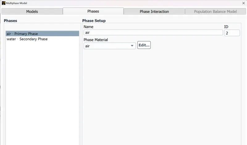
Then we create the materials as air and water.

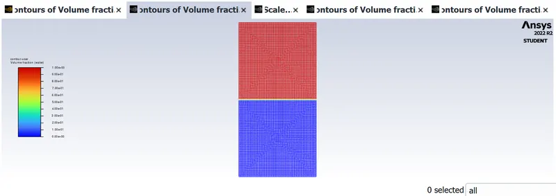
Next step is the initialization of the solution and then we create the patch values alpha as 0 for air and 1 for water.

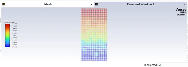
Then we create the plot and animation.The contour will be as shown below, with red coloured part as 1 and blue as 0.

RESULTS

The solution for the baseline set up with mesh size of 0.5mm, 300 time steps

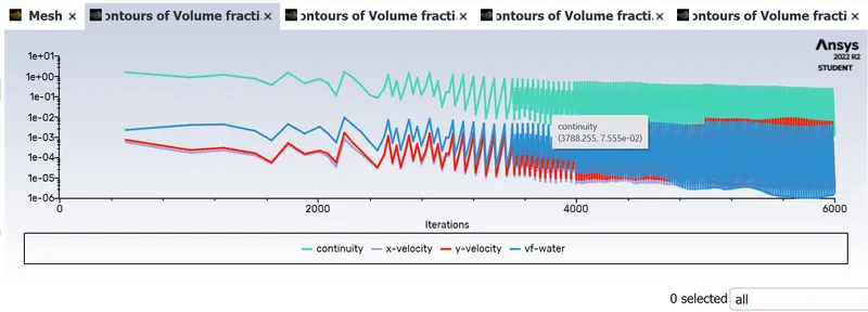
Residuals

Animation

https://drive.google.com/file/d/1qc9rOjpRdZT5hK_PQ0TYbZ6aMxytg48C/view?usp=share_link

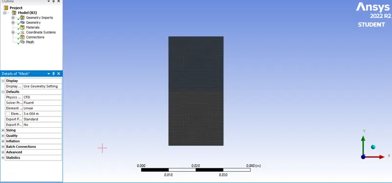
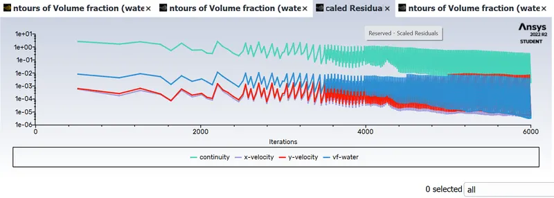
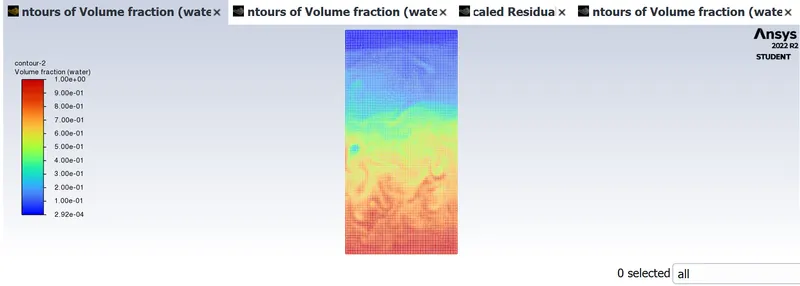
Case 2: For mesh size of 0.3 mm and 300 time steps

Mesh

Residuals

Animation

 https://drive.google.com/file/d/1-SOSRiTm3YHTN-0SZk8hFUlXM9Tl8oi4/view?usp=share_link

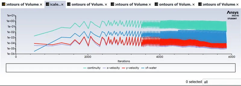
Case 3 : Using water and user defined material with viscosity 0.001 kg/ms and density 400 kg/m^3 and with element size 0.3 mm for 300 time steps

Residuals

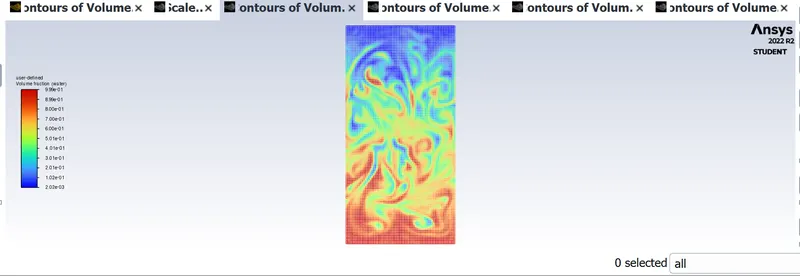
Animation

https://drive.google.com/file/d/1l0XsCEDOczjQXFQQNt6arX7nFfDNK87C/view?usp=share_link

Atwood Number:

• The Atwood number is a dimensionless number in fluid dynamics used in the study of hydrodynamic instabilities in density stratified flows.
• It is a dimensionless density ratio related to the density of heavier fluid and the density of lighter fluid. (The difference in the fluid densities divided by their sum).
• Atwood number is an important parameter in the study of Rayleigh–Taylor instability.
• For Atwood number close to 0, RT instability flows take the form of symmetric “fingers” of fluid;
• for Atwood number close to 1, the much lighter fluid “below” the heavier fluid takes the form of larger bubble-like plumes.

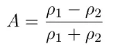
  A = Atwood number 

`rho1`= density of heavy fluid

`rho2`= density of lighter fluid

So Considering above Cases we can calculate the atwood number by using the above formula

So using the above formula we get Atwood NUmber as

Case 1 and Case 2 = 0.99754 

Case 3 = 0.4285

CONCLUSION

Here we can conclude that 

• Higher the atwood Number the Instabilites are sudden and Reach steady state more rapidly
• Lower the Atwood Number Instabilites Take time and Reach steady state slowly
• From the animation video it is able to visualize the RT instability of two fluid accurately. It is also concluded that fine meshing provide a clear picture of simulation as compared to baselinemeshing. 

RTI evolves in three distinct stages:

• Linear stability,
• mushroom head(falling) or bubble(rising) formation,
• long term evolution due to bubble merging and mixing.

For low Atwood number, bubble and mushroom head shape is relatively symmetrical, the disturbances or perturbations are linear for a larger time. 

for large Atwood number, bubble and mushroom head shape is less symmetrical, also it occurs very rapidly at an accelerating rate which leads to a nonlinear growth rate.

Why Steady State simulation is not suitable ?

• We know that steady state simulation is a time independent approach. 
• Based on the simulation we know there is high turbulence involved and the change in the flow occurs between very small time variation. This is not possible to capture in steady state solution
• Also steady state solver ignore the time differential terms involved in the simulation and thus even if it may be able to capture the state of equilibrium, it skips to capture the non-linearities in the simulation precisely.
• Since the simulation involves capturing instabilities that are changing in an unpredictable manner as a function of time, the transient approach is preferred over the steady-state approach.