Week 5 - Rayleigh Taylor Instability
Rayleigh Taylor Instability:
Rayleigh-Taylor instability is the interpenetration of materials that occurs whenever a light fluid pushes on a heavy fluid. It is a dynamic process whereby the two fluids seek to reduce their combined potential energy.
Different CFD models that are based on the mathematical analysis of Rayleigh Taylor waves-
1. Kelvin Helmholtz Instability Model -
When there is velocity shear in a single continuous fluid or when there is a velocity differentce across the interface between two fluids, the Kelvin-Helmholtz instability can happen. : The instability occurs as waves on the water surface, in the clouds, the ocean, Saturn's bands, and the sun's corona show this instability.
2. Richtmeyer-Meshkow Instability -
The Richtmyer-Meshkov instability arises when a shock wave interacts with an interface separating two different fluids. It combines compressible phenomena, such as shock interaction and refraction, with hydrodynamic instability, including nonlinear growth and subsequent transition to turbulence, across a wide range of Mach numbers.
3. Plateau–Rayleigh instability-
The Plateau–Rayleigh instability, explains why and how a falling stream of fluid breaks up into smaller packets with the same volume but less surface area. The driving force of the Plateau–Rayleigh instability is that liquids, because of their surface tensions, tend to minimize their surface area.
Rayleigh Taylor instability simulation:
Case1-
Modeling
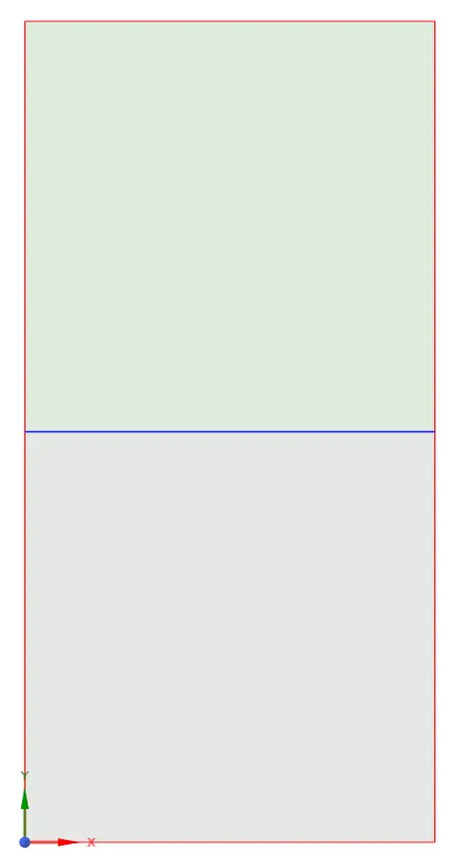
The model is a rectangular surface that is created with two squares one on top of another. The squares are of 20mm and that share a single common edge. For this, shared topology was enabled.
Meshing-
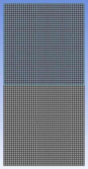
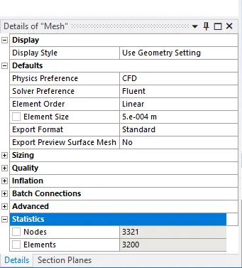
I created a baseline mesh of size 0.5mm
Simulation Setup-
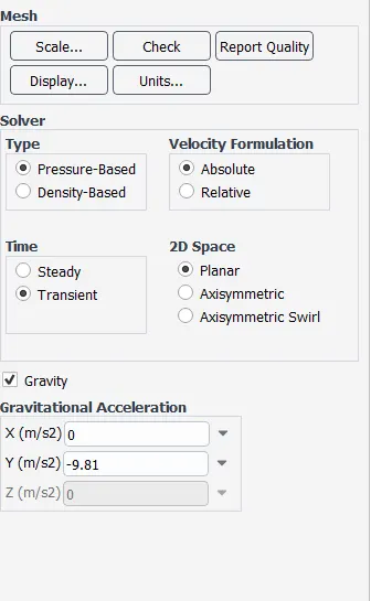
For this scenario, the solver type is pressure based with time as transient. Gravity was enabled at -Y direction with a value of 9.81m/sec
The solver used is Viscous - Laminar
Materials used -
Air:
Density = 1.225 kg/m^3
Viscosity = 1.7894e-05 kg/m-s
Water:
Density = 998.2 kg/m^3
Viscosity = 0.001003 kg/m-s
Multiphase model properties-
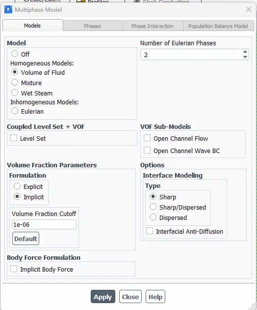
After standard initialization, patches have to be created for both volumes to assign respective materials. A volume fraction of 1 was assigned to water and 0 to air and user defined material.
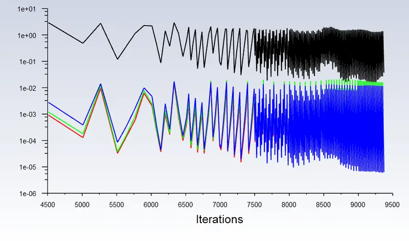
The simulation was run with time step 0f 0.002 for 500 iterations.
Case 1 results-
Case 2-
A mesh size of 0.3mm was given.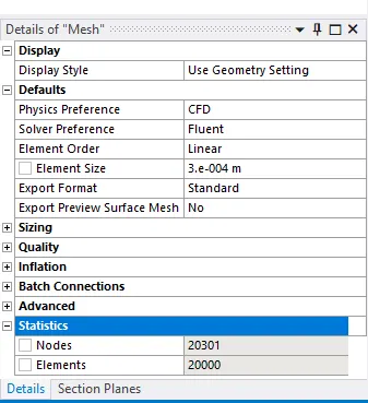
This setup was solved for 1000 iterations with time step value as 0.002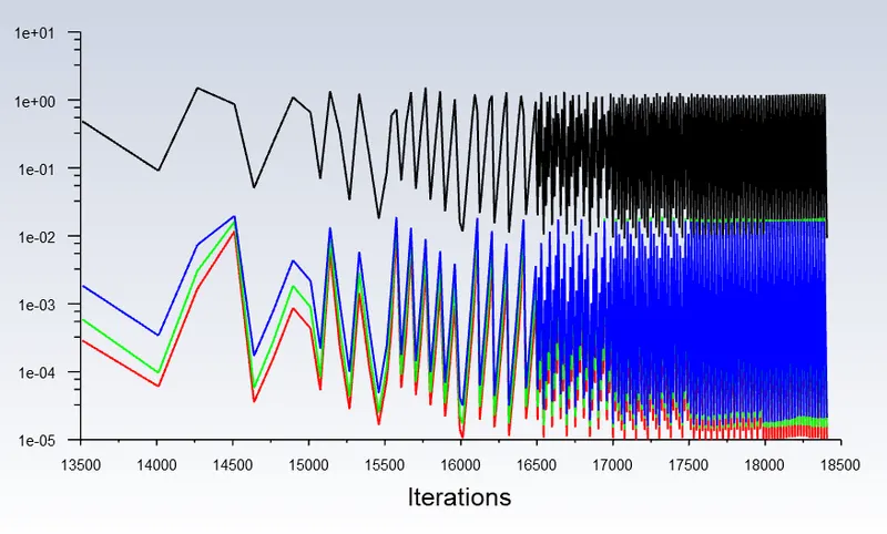
Case 3-
A mesh size of 0.2mm was given.
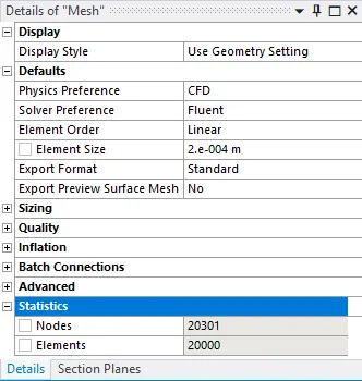
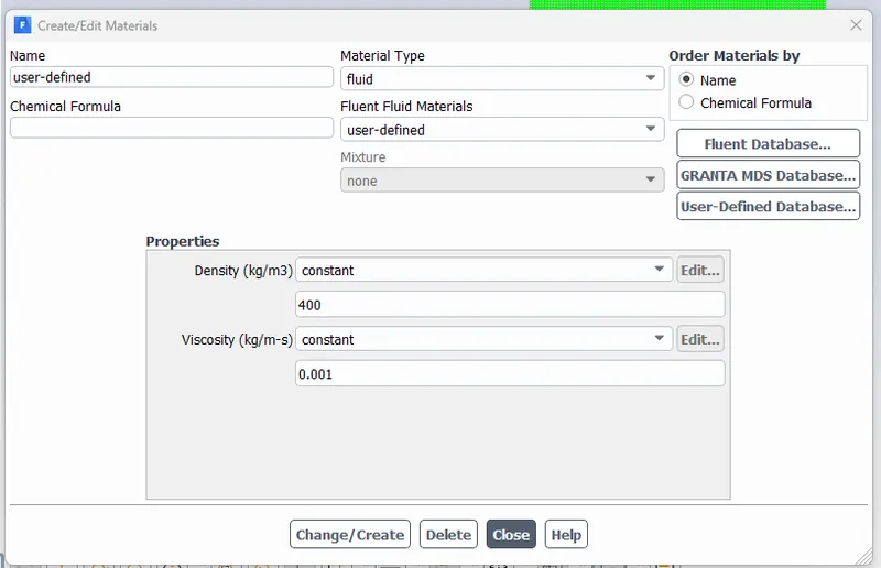
Materials used-
User defined:
Density = 400 kg/m^3
Viscosity = 0.001 kg/m-s
Water:
Density = 998.2 kg/m^3
Viscosity = 0.001003 kg/m-s
This setup was solved for 1000 iterations with time step value as 0.002
Instability animations for all 3 cases-
https://drive.google.com/drive/folders/1ZLFeOLDv8KtF_eh-pS_cLEn7qwsG2BTt?usp=share_link
Observation-
A transient approach was selected in order to observe the equilibrium state between the two fluids. Also, the velocities of the fluids are unknown and the flow patterns are irregular and unpredictable.
The instabilities can be better observed in the case of finer mesh. The finer the mesh, the longer it takes for the program to solve. Finer mesh yields more accurate results at the expense of time. As the higher density flud (water) starts to flow into the lower volume due to gravity, formation of air bubbles and vortices are observed, which travels towards the upward region with time until it reaches an equilibrium.
Atwood Number-
The Atwood number is a dimensionless number in fluid dynamics used in the study of hydrodynamic instabilities in density-stratified flows. It describes the density difference between two adjacent fluids with a common interface.
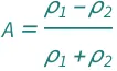
For Air and Water-
A = (998.2-1.225)/(998.2+1.225)
A = 0.998
For Water and User defined material-
A = (998.2-400)/(998.2+400)
A=0.428
For the case with user defined fluid, the density is higher than air. Hence the water takes a longer time to achieve equilibrium.