Week 5 - Rayleigh Taylor Instability
Aim :- To perform Rayleigh Taylor instability simulation by using two diffrent material and one more simulation with user define material (density = 400 kg/m3, viscosity = 0.001 kg/m-s). Define Atwood number.
Some pratical CFD models based on the mathematical analysis of Rayleigh
Taylor waves are :
Rayleigh Taylor Instability -
It is an instability of an interfaces between two fluids of different densities which occurs
when the lighter fluid is pushing the heavier fluid.
Kelvin Helmholtz Instability Model -
This instability can occur when there is velocity shear in a continous fluid, or where there is a velocity difference across the interface between two fluids. An example is Wind blowing over the water. Other examples showing this instability are clouds, oceans, Saturn\'s bands, Jupiter\'s Red Spot and more famously the Sun\'s Corona.
Richtmeyer-Meshkow Instability -
This instability occurs when a shock wave interacts with an interface separating two different fluids or in other words when two fluids of different densities are impulsively accelerated.The development of instabitlity begins with small amplitude perturbations which initially grow linear with time. This instability can be considered the impulsive acceleration limit of the Rayleigh-taylor instability.
Plateau-Rayleigh Instability -
This instability explains why and how a falling stream of fluid breaks up into smaller packets with the same volume but different or small surface area. It is often called as Rayleigh Instability. The driving force of this instablity is that the liquids by virtue of their surface tensions, tend to minimize their surface area.
Solution and results:-
In this project, we consider 3 different cases in which 2 cases are based on the type of MESHING and the other is with user-defined materials. We consider 2 materials air and water placing one above the other and see the effect of gravity acting on them.
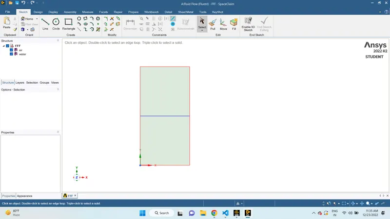
Geometry :- For our project, we consider a simple 2D geometry of which
- We draw 2 squares one above the other with a length of 0.02 m.
- Then naming the below square as air and above square as water in 2 different components.
- And share the topology for a perfect intersection between both surfaces.
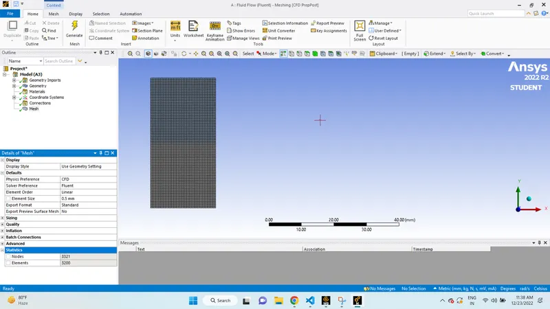
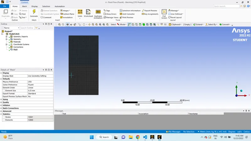
Mesh :- Overall mesh size is 0.5 mm
Setup and solver :-
solver - pressure based
time - transient
gravity - -9.81 (in y direction)
viscous model - laminar
fluid type - air , water liquid
multiphase - volume of fluid > implict > phase 2
initialization - standard (with transient time)
patch - water>volume of fraction>for water use 1 and for air use zero.
make contour - phase> water
create solution animation at contour
simulation run for 0.025 to 100 time steps
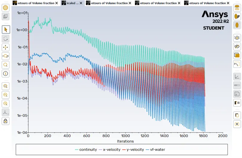
Residuals :-
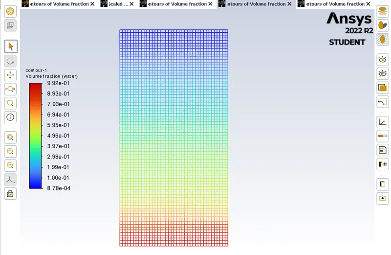
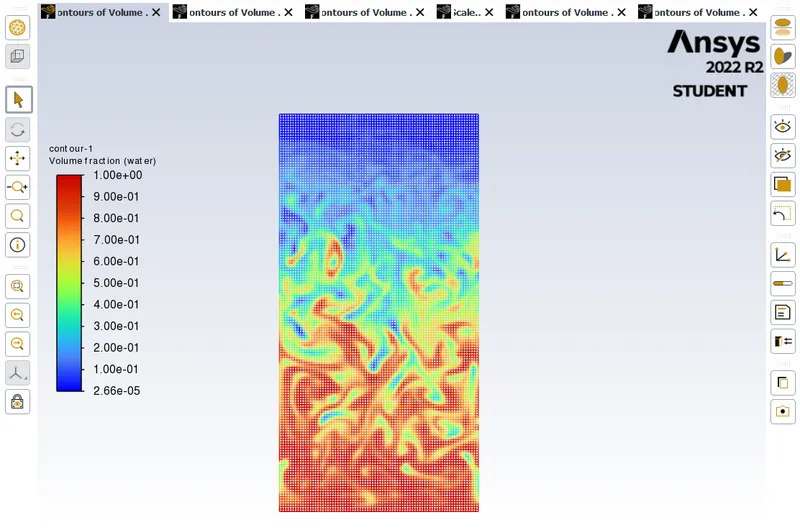
Contours of volume fraction :-
Mesh :- (refined)
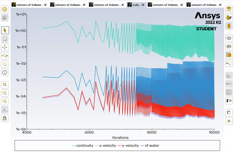
overall mesh size 0.25 mm and calculation run for the 0.002 to 500 time steps
Residuals :-
Contours :-
Link :- https://drive.google.com/file/d/107ZoKqLsTuM2M3M78vvyXk12pZFHSwDc/view?usp=share_link
Mesh :-
same as previous mesh but material change with user defined material
user-defined material - density = 400 kg/m3, viscosity = 0.001 kg/m-s
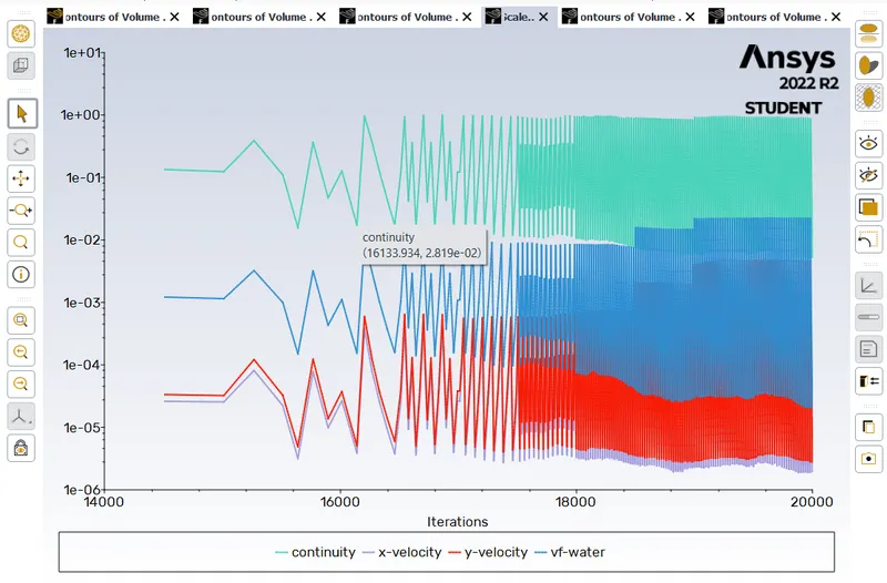
calculation run for the 0.002 to 500 time steps
Residuals :-
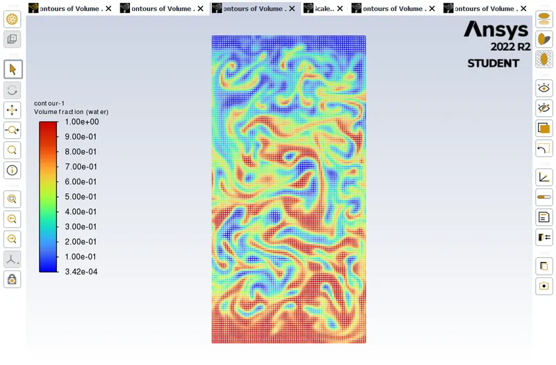
Contours :-
Atwood number :-
The Atwood number (A) is dimensionless in fluid dynamics used in the study of hydrodynamic instabilities in density stratified flows. It is a dimensionless density ratio defined as

where
 = density of heavier fluid
 = density of the lighter fluid
In Rayleigh–Taylor instability, the penetration distance of heavy fluid bubbles into the lighter fluid is a function of the acceleration time scale,  where g is the gravitational acceleration and t is the time.
A = `(rho1-rho2)/(rho1+rho2)`
A =`(998.2 − 1.225)/( 998.2 + 1.225)`
A = 0.9975
Conclusion :-
- Since the simulation involves capturing instabilities that are changing in an unpredictable manner as a function of time, the transient approach is preferred over the steady-state approach.