Week 5 - Rayleigh Taylor Instability

Rayleigh Taylor Instability

Aim:To perform the Rayleigh Taylor instability simulation

Objectives:

1. To explain some practical CFD models that have been based on the mathematical analysis of Rayleigh Taylor waves.
2. To perform the Rayleigh Taylor instability simulation for 2 different mesh sizes with the base mesh being 0.5 mm.
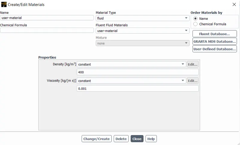
3. To run one more simulation with water and user-defined material(density = 400 kg/m³, viscosity = 0.001 kg/m-s) for refined mesh.
4. To define the Atwood Number and to find out the Atwood number for both the cases and explain how the variation in Atwood number in the above two cases affects the behavior of the instability.

Theory:

Rayleigh–Taylor instability (or RT instability) is named after Lord Rayleigh and G. I. Taylor. There are situations where a heavy liquid layer is placed over a lighter fluid layer. This situation has engineering implications in several industries. For example in die casting, liquid metal is injected in a cavity filled with air. In poor designs or other situations, some air is not evacuated and stay in small cavity on the edges of the shape to be casted. Thus, it can create a situation where the liquid metal is above the air but cannot penetrate into the cavity because of instability. This instability deals with a dense, heavy fluid that is being placed above a lighter fluid in a gravity field perpendicular to interface. Example for such systems are dense water over oil (liquid–liquid), or water over air(gas–liquid).

• Practical CFD models that have been based on mathematical analysis of RT waves:

1. Kelvin-Helmholtz instability
2. Richtmyer-Meshkov instability
3. Plateau-Rayleigh instability

Kelvin-Helmholtz instability: This instability typically occurs when there is velocity shear in a single continuous fluid, or additionally where there is a velocity difference across the interface between two fluids. A common example is seen when wind blows across a water surface; the instability constant is able to manifest itself through waves on water surface. The Kelvin-Helmholtz instability is not only restricted to a water surface as clouds, but is evident through other natural phenomena as ocean and the sun's corona.

Richtmyer-Meshkov instability:This occurs when two fluids of different density are impulsively accelerated. Normally this is by the passage of a shock wave. The development of the instability begins with small amplitude perturbations which initially grow linearly with time. This is followed by a nonlinear regime with bubbles appearing in the case of a light fluid penetrating a heavy fluid, and with spikes appearing in the case of a heavy fluid penetrating a light fluid. A chaotic regime eventually is reached and the two fluids mix. This instability can be considered the impulsive-acceleration limit of the Rayleigh Taylor instability.

Plateau-Rayleigh instability:This instability, often just called the Rayleigh instability, explains why and how a falling stream of fluid breaks up into smaller packets with the same volume but less surface area. It is related to the RTI and is part of a greater branch of fluid dynamics concerned with fluid thread breakup. This fluid instability is exploited in the design of a particular type of ink jet technology whereby a jet of liquid is perturbed into a steady stream of droplets. The driving force of the Plateau–Rayleigh instability is that liquids, by virtue of their surface tension, tend to minimize their surface area.

Modelling and solving:

Geometry creation:

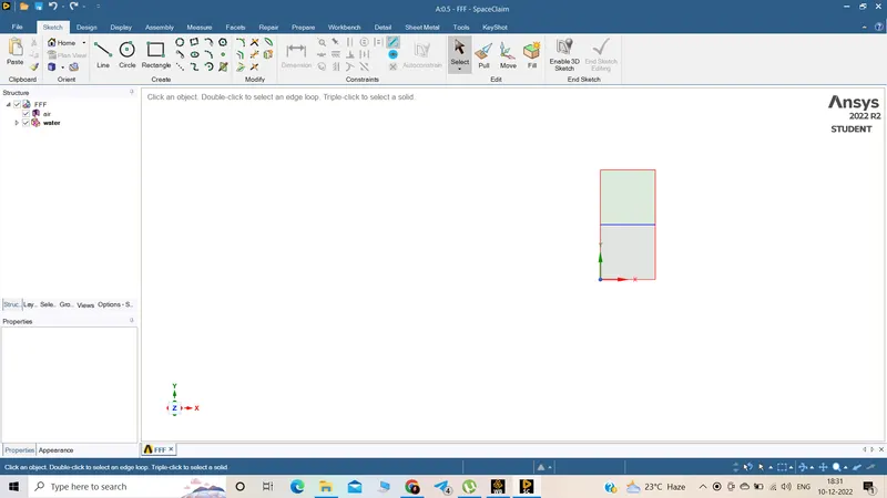
• Create 2 rectangles of size 20x20 mm, lower one of air & upper one for water.
• Create conformal mesh to have common interface between 2 interface & to share information.

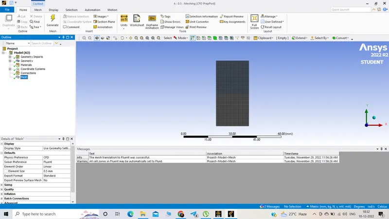
Meshing with baseline mesh 0.5mm:

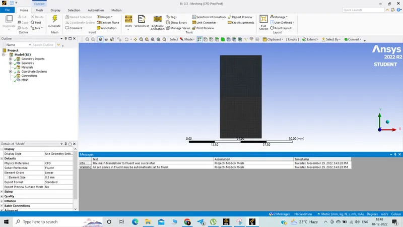
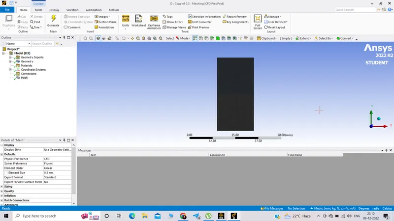
Meshing with refined mesh 0.3mm:

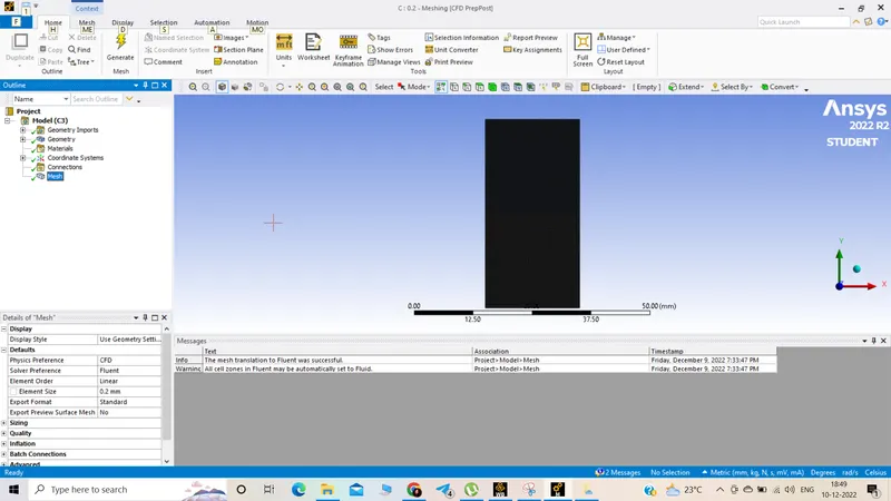
Meshing with refined mesh 0.2mm:

Set up:

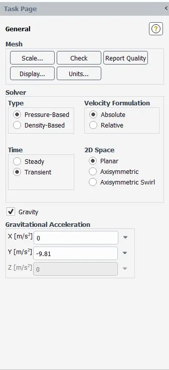
General:

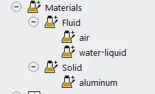
Materials:

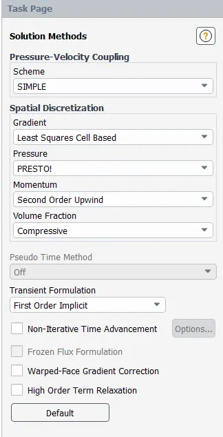
Methods:

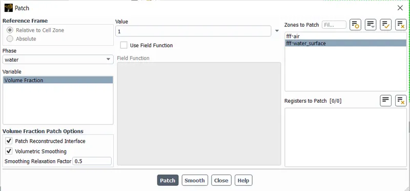
initialized the solution and patch:

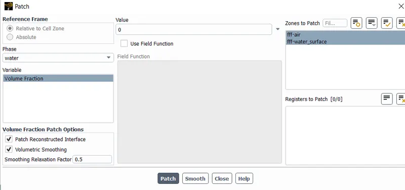
Create contour and animation

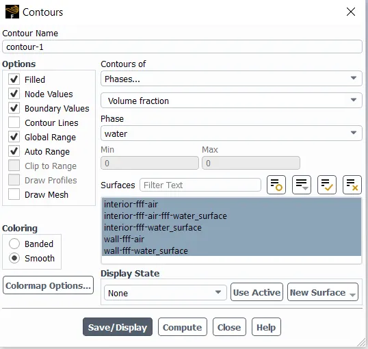
Create animation of this contour.

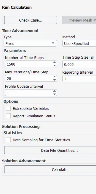
Run calculation:

Result:

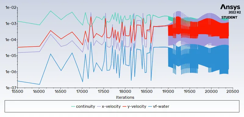
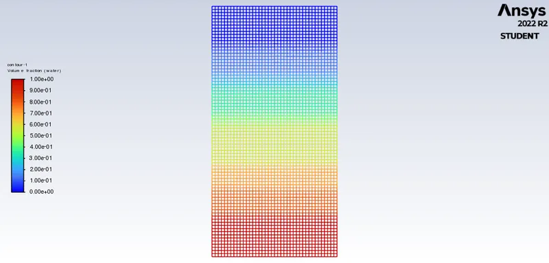
Meshing with refined mesh 0.5mm:

Residuals

Contour of volume fraction:

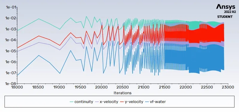
Meshing with refined mesh 0.3mm:

Residuals

Contour of volume fraction:

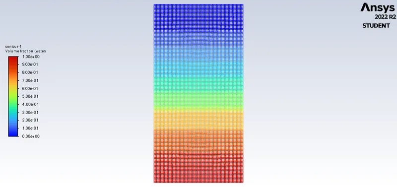
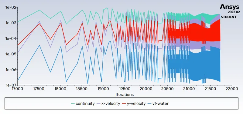
Meshing with refined mesh 0.2mm:

Residuals

Contour of volume fraction:

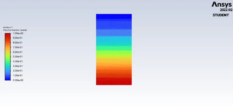
Meshing with refined mesh 0.3mm and user material-water:

Mesh:

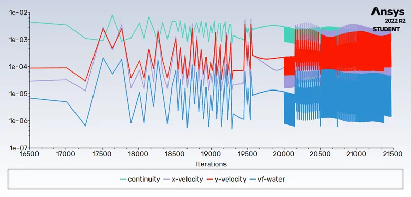
Residuals:

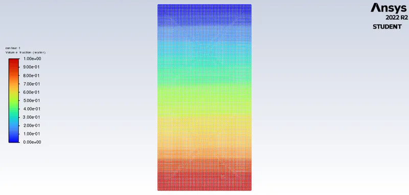
Contour of volume fraction:

Adding user -material:

Animations :

Animation1: for 0.5 mm air water

Animation2: for 0.3 mm air water

Animation3: for 0.2 mm air water

Animation4: for 0.3 mm user material water

https://drive.google.com/drive/folders/1a6R05qtV0T9zXIoljFv_vehfUujaEC7n?usp=share_link

Observations:Finer mesh captures the instability better than the coarse mesh , but it takes more time for the heavier fluid to settle down. So it is computationally expensive but produces results with better accuracy.

Reason for a steady-state approach might not be suitable for these types of simulation:

The steady-state simulation is performed if we are concerned more about the final state results or the equilibrium state. In RT-Instability CFD models, we are more concerned to learn about the transition of the irregularities that starts developing when we pour high dense fluid upon low dense fluid under gravity effect so, by using transient solver along with refined mesh of the model, we can compute the smooth transition of irregularities that takes place at the interface of the fluids. The final state results for both the steady-state and transient state will be the same.We want to see how the interface collapses as a function of time.

Atwood Number:

The Atwood number is a dimensionless number in fluid dynamics used in the study of hydrodynamic instabilities in density stratified flows. It is a dimensionless density ratio related to the density of heavier fluid and the density of lighter fluid. (The difference in the fluid densities divided by their sum). Atwood number is an important parameter in the study of Rayleigh–Taylor instability. For Atwood number close to 0, RT instability flows take the form of symmetric “fingers” of fluid; for Atwood number close to 1, the much lighter fluid “below” the heavier fluid takes the form of larger bubble-like plumes.

A	Atwood number (dimensionless)
ρ1	Density of heavier fluid (kg/m3)
ρ2	Density of lighter fluid. (kg/m3)

`A=(rho_1-rho_2)/(rho_1+rho_2)`

For Air-water RT instability:

ρ₁ = 998.2 kg/m³ [Water density]

ρ₂ = 1.225 kg/m³ [Air density]

A = (998.2-1.225)/(998.2+1.225)

A = 0.998 (the much lighter fluid “below” the heavier fluid takes the form of larger bubble-like plumes.)

For usermaterial-water RT instability:

ρ₁ = 998.2 kg/m³ [Water density]

ρ₂ = 400 kg/m³ [Usermaterial density]

A = (998.2-400)/(998.2+400)

A = 0.428 ( flows take the form of symmetric “fingers” of fluid)

Conclusion:Atwood number forms a basis to compare the RT Instabilty. The calculated Atwood numbers are validated with simulation results.