Week 5 - Rayleigh Taylor Instability

Aim

To perform the Rayleigh Taylor instability simulation for the two different cases :

1. Rayleigh-Taylor instability simulation for air and water

2. Rayleigh-Taylor instability simulation for water and user-defined material(density = 400 kg/m³, viscosity = 0.001 kg/m-s)

To find the Atwood number for both the cases.

Introduction

some practical CFD models that have been based on the mathematical analysis of Rayleigh Taylor waves :

Plateau-Rayleigh instabiity

Explains why and how a falling stream of fluid breaks up into smaller packets with the same volume but less surface area. It is related to the Ryleigh- Taylor instability. and is part of a greater branch of fluid dynamics concerned with fluid thread breakup. This fluid instability is exploited in the design of a particular type of inkjet technology. whereby a jet of liquid is perturbed into a steady stream of droplets. The driving force of the Plateau–Rayleigh instability is that liquids, by virtue of their surface tensions, they tend to minimize their surface area.

Kelvin-Helmholtz instability

This instability occurs where there is a velocity shear or velocity difference between the interface of the multiphase fluids.

Richtmyer-Meshkov instability

Instability occurs when there is an impulsive acceleration between the two fluids. This type of instability can occur when there is a shock at greater speeds.

Solving and modelling approach

The work flow to perform the Rayleigh-Taylor instability simulation :

• Pre-processing
• Solving
• Post-processing

In pre-processing the geometry is modelled with help of spaceclaim provided in the Ansys workbench.

After which mesh generation is carried out for the geometry.

Using ansys fluent some of the solver requirements are taken care such as setting up physics and setting up the solution.

End results are visualized in the post-processing such as contour plots, line plots, vector plots and solution animation.

A steady-state approach might not be suitable for these type of simulation because in steady-state approach it dose not depend on time and it will generate only the end results of the simulation. There is no possiblity to see the instability occurred during mixing of air and water. Thus the trasient simulation is simulated with respect to time in order to view the instability which is occured during mixing.

Pre-processing

Geometry

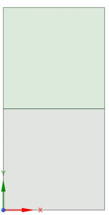
Initial geometry which is created using spaceclaim. It has two different surfaces.

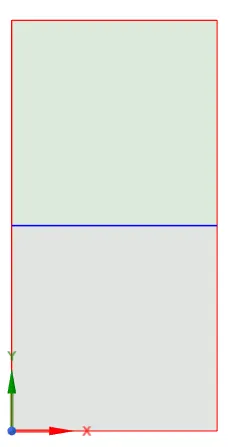
Final geometry after enabling share topology.

Mesh

Mesh is generated after modelling.

Case 1 : Baseline mesh - element size of 0.5 mm

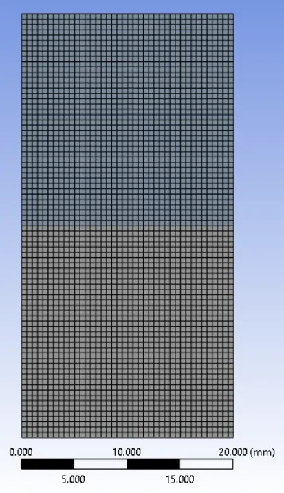
Element size = 0.5 mm

Number of elements = 3200

Case 2 : Refined mesh size of 0.1 mm

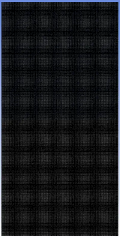
Element size = 0.1 mm

Number of elements = 80000

Solver settings

Setting up physics

Pressure based transient solver is used.

Velocity formulation is absolute and the gravity is enabled and set to -9.81 m/s²

Viscous model is set to laminar.

In multiphase model, model is set to volume of fluid with implicit formulation.

Primary phase is air where as secondary phase is water for the case 1 and case 2 simulation and for the case 3 simulation primary phase is user-defined material (density = 400 Kg/m³, viscosity = 0.001 Kg/m-s) and secondary phase is water.

Setting up the solution

Solution is initialized using hybrid initialization.

Using the patch option the volume fraction for the water is one and for the air it is zero.

Results

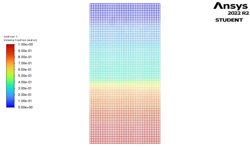
Case 1 : Baseline mesh - element size used is 0.5 mm (Air and water)

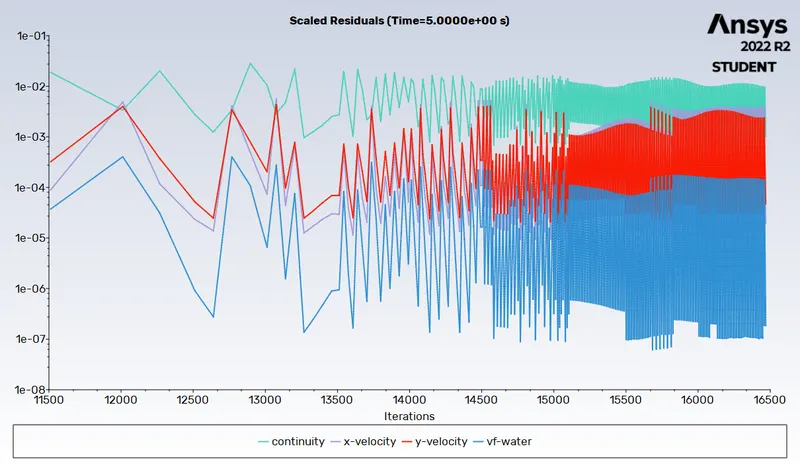
Residuals

Contours

Animation

https://drive.google.com/file/d/1e03SeRiZYgoNR2uHd3XPaCToLuuq_mVH/view?usp=share_link

Case 2 : Refined mesh - element size used is 0.1 mm (Air and water)

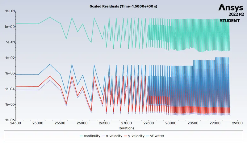
Residuals

Contours

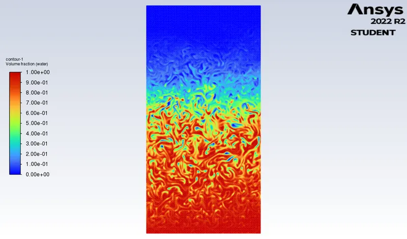
The instability which is occured during mixing of air and water can be visualized clearly for refined mesh compared to the baseline mesh.

Animation

https://drive.google.com/file/d/1vseMIpdmwAIOd2xDAYoHSA-5x0rXEwJy/view?usp=share_link

Case 3 : Refined mesh - element size used is 0.1 mm, water and user-defined material(density = 400 kg/m³, viscosity = 0.001 kg/m-s)

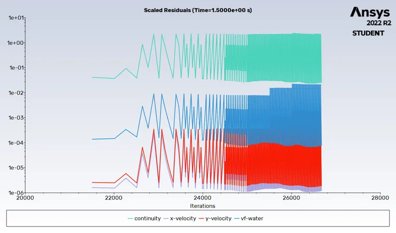
Residuals

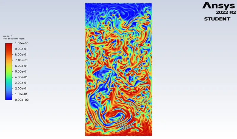
Contours

Animation

https://drive.google.com/file/d/1sdmq47ehgeNXsGuXvtvezF6cgClvNzki/view?usp=share_link

Atwood Number

Atwood number is a dimensionless number which describes the density difference between the two adjacent fluids with a common interface.

Atwood number is an important parameter in the study of Rayleigh-Taylor instability and Richtmyer-Meshkov instability. In Ratleigh-Taylor instability, the penetration distance of heavy fluid bubbles into the light fluid is a function of acceleration time scale, Agt². Where 'g' is the gravitational acceleration and 't' is the time.

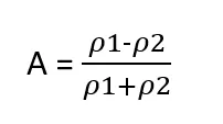
Where,

A = Atwood number

ρ1 = Density of heavier fluid

ρ2 = Density of lighter fluid

Case 2 : Refined mesh - element size used is 0.1 mm (Air and water)

ρ1 = Density of water = 998.2 Kg/m³

ρ2 = Density of air = 1.225 Kg/m³

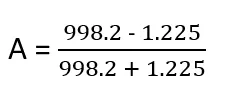
A = 0.997

Case 3 : Refined mesh - element size used is 0.1 mm, water and user-defined material(density = 400 kg/m³, viscosity = 0.001 kg/m-s)

ρ1 = Density of water = 988.2 Kg/m³

ρ2 = Density of user-defined material = 400 Kg/m³

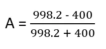
A = 0.427

For Atwood number close to 0, Rayleigh-Taylor instability takes the form asymmetric 'finger' of fluid.

For Atwood number close to 1, the much lighter fluid 'below' the havier fluid takes the form of larger bubble-like plumes.

Conclusion

The calculated Atwood number is close to 1. From the simulation results it is found that when high dense fluid water poured upon low dense fluid air under gravity, the formation of air bubble-like plumes takes place which travels towards the upward region in the form of waves and some gets trapped at the lower region during initial stages which afterwards try to move towards the upper region and at the end, both phases gets separated with some diffusivity left at the middle portion between them.