Week 5 - Rayleigh Taylor Instability

AIM -

A transient state simulation is to be performed to study the Rayleigh Taylor Instability phenomenon in Ansys Fluent.

INTRODUCTION -

The Rayleigh-Taylor instability occurs when the lighter fluid pushes the heavier fluid across an interface between two fluids of different densities. Water suspended over oil, for example, can be represented by two entirely plane-parallel layers of immiscible fluid, the denser fluid on top of the less dense one, both subject to Earth's gravity.

If a parcel of heavier fluid is displaced downward with an equal volume of lighter fluid displaced upwards, the potential energy of the configuration is lower than the initial state. Thus the disturbance will grow and lead to a further release of potential energy, as the denser material moves down under the gravitational field, and the less dense material is further displaced upwards. This phenomenon occurs deep underwater on the surface of an expanding bubble and in a nuclear explosion.

In fluid dynamics, the Atwood number (A) is a dimensionless number that is used to examine hydrodynamic instabilities in density-stratified flows. It is a dimensionless density ratio that is calculated as the ratio of the difference in fluid densities to the sum of those densities.

`A = frac{rho_1-rho_2}{rho_1+rho_2}`

where

`rho_1`= density of heavier fluid

`rho_2`= density of lighter fluid

The Rayleigh Taylor instability flows appear as symmetric fingers of fluid for A close to 0, whereas for A close to 1, the much lighter fluid below the heavier fluid appears as bigger bubble-like plumes.

This process can be seen in a number of examples on Earth, such as salt domes and weather inversions, as well as in astrophysics and electrohydrodynamics. For instance, the Crab Nebula, which is being swept up by an expanding pulsar wind nebula propelled by the Crab pulsar, exhibits a Rayleigh-Taylor instability structure. This supernova explosion occurred 1000 years ago. Recent research has also shown that RT instability occurs when a relatively dense solar prominence stands on top of a less dense plasma bubble in the solar corona, the Sun's outer atmosphere. The latter instance is comparable to RT instabilities with magnetic modulation.

Rayleigh Taylor waves are associated with some instability patterns, like as;

1. Saffman–Taylor Instability -

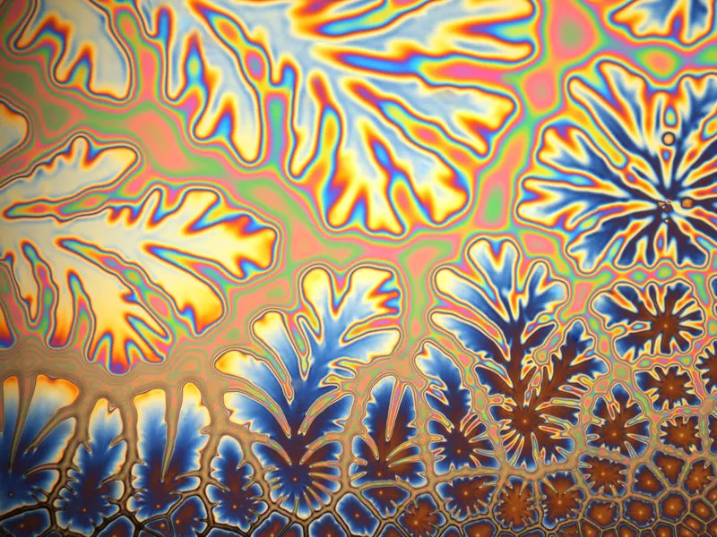
The Saffman-Taylor instability, or viscous fingering, is the development of patterns at a morphologically unstable interface between two fluids in a porous medium. The process of draining media, such as soils, most frequently brings about this scenario. When a more viscous fluid is displaced by a less viscous fluid, the interface becomes unstable. If the opposite occurs, however, with the more viscous fluid displacing the less viscous, no instability is observed.

2. Richtmyer-Meshkov Instability -

When two fluids with different densities are accelerated abruptly, the Richtmyer-Meshkov instability (RMI) develops. Usually, a shock wave will pass through to do this. Small amplitude perturbations that first increase linearly with time are the beginning stages of the instability's development. After that, a nonlinear regime sets in, where bubbles occur when a light fluid penetrates a heavy fluid, and spikes appear when a heavy fluid penetrates a light fluid. The two fluids eventually combine as a chaotic regime. This instability can be considered as the Rayleigh-Taylor instability's impulsive-acceleration limit.

3. Kelvin-Helmholtz Instability -

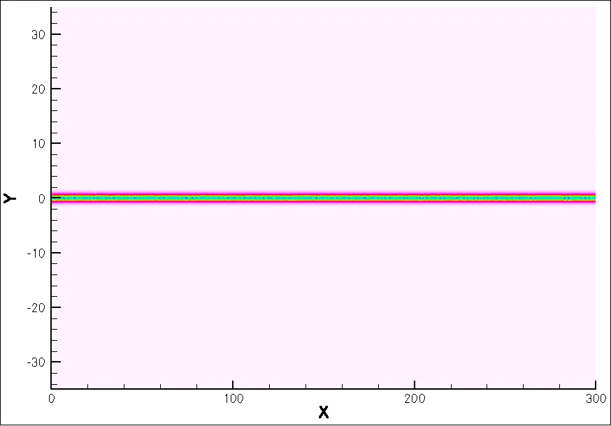
When there is velocity shear in a single continuous fluid or a velocity difference across the interface between two fluids, the Kelvin-Helmholtz instability, a fluid instability, happens. The atmospheres of planets and moons, such as the Red Spot on Jupiter or the Earth's clouds, as well as the atmospheres of the Sun and other stars, exhibit Kelvin-Helmholtz instabilities.

4. Kármán Vortex Street -

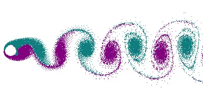
The uneven separation of flow of a fluid around blunt bodies is induced by a process known as vortex shedding, which results in the Kármán Vortex Street, a pattern of swirling vortices.

The above instabilty models can be used to perform CFD calculations.

THEORY -

• Multiphase:-

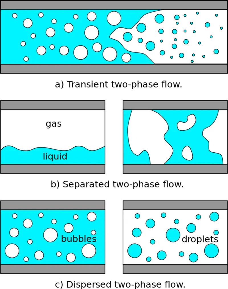
In both nature and technology, there are many flows that are a combination of stages. The three physical phases of matter are gas, liquid, and solid, but in a multiphase flow system, the term "phase" is used in a much broader sense. A phase in a multiphase flow is an identified type of material that interacts and responds inertially in a specific way to the flow and the potential field it is submerged in. For instance, since any collection of particles with the same size would have a comparable dynamical reaction to the flow field, different-sized solid particles of the same material can be considered as different phases.

Types of phases in Multiphase -

1. A separated phase is defined as one or more immiscible fluids in a continuous phase separated by an interface.
2. The dispersed phase is defined as the phase in which a finite number of phases are spread in a continuous phase.
3. A mixed phase is defined as the phase in which one or more fluids are mixed. It contains both the separate and dispersed phases.

• VOF Model:-

The VOF model is a surface-tracking technique applied to a fixed Eulerian mesh. It is designed for two or more immiscible fluids where the position of the interface between the fluids is of interest. In the VOF model, a single set of momentum equations is shared by the fluids, and the volume fraction of each of the fluids in each computational cell is tracked throughout the domain. Applications of the VOF model include stratified flows, free-surface flows, filling, sloshing, the motion of large bubbles in a liquid, the motion of liquid after a dam break, the prediction of jet breakup (surface tension), and the steady or transient tracking of any liquid-gas interface.

Let us consider `alpha = phase 1`, and `beta = phase 2` then, VOF should be `alpha + beta = 1`

• Transient State:-

The VOF formulation in Ansys Fluent is generally used to compute a time-dependent solution, but for problems in which you are concerned only with a steady-state solution, it is possible to perform a steady-state calculation. A steady-state VOF calculation is sensible only when your solution is independent of the initial conditions and there are distinct inflow boundaries for the individual phases. For example, since the shape of the free surface inside a rotating cup depends on the initial level of the fluid, such a problem must be solved using the time-dependent formulation. On the other hand, the flow of water in a channel with a region of air on top and a separate air inlet can be solved with the steady-state formulation.

1. Explicit scheme - It offers time-accurate data, but time step size must be taken to ensure that the Courant number is satisfied.

2. Implicit scheme - It will offer the speed of the steady state but will need a time-varying solution. It is unconditionally stable, and it is the default stable analysis fluent. Timestep size is not the constraint in this scheme.

When compared to steady-state simulation, transient simulation has a larger processing time need. A transient solver can be utilized to operate at fewer time steps and capture the flow better. The only way to examine the instabilities at smaller time scales is through transient simulation. Transient simulation is the best configuration to do the computation for Rayleigh Taylor Instability since it is a time-marching solution, which calls for greater accuracy.

• Courant Number:-

It is a non-dimensional number that represents how quickly information moves through a discretized domain. The courant number is the ratio of these two lengths or the fraction of the cell traveled by the flow in a time step. The time step size for explicit integration must be less than a particular value or the solution will be incorrect.

`Total Flow Time = Timestep size xx Number of Timesteps`

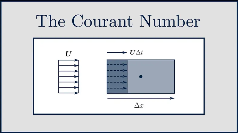`Co = frac{Len. Fluid}{Len. Cell} = frac{U Delta t}{Deltax} gt 1`


SOLVING & MODELLING APPROACH -

For three cases, the simulation will be executed. In the first two scenarios, water is placed above air because it is heavier and denser. We will utilize coarse mesh (0.5 mm) in the first case, and refined mesh in the latter case (0.1 mm). In the third case, the simulation will be done using water and a user-defined material with the following properties: density`(400(kg)/m^3)`, viscosity `(0.001(kg)/(mcdot s))`, implementing a fine mesh (0.1 mm).

We'll utilize the "Transient state" as the solver time in this simulation investigation. However, it is divided into two schemes: the explicit scheme and the implicit system. We will utilize Ansys Fluent's Implicit scheme, which is the default scheme and does not have a timestep size restriction, for our simulations. In an explicit approach, we must first compute the courant number and then choose the timestep size in accordance with that result. In implicit formulation, the solution information propagates much faster compared to the explicit formulation. Following the Atwood number calculation, we will make relevant conclusions based on the results of the simulation.

Double-click the 'Fluid Flow (Fluent)' system in the Ansys Workbench. Modify the system's name to 'Case 1'.

PRE-PROCESSING -

To start SpaceClaim, right-click the 'Geometry' file.

In this section, we will create a two-dimensional domain for the fluids in the XY plane. The simulations will be performed in this domain.

Select 'Sketch Mode,' then click the cursor in the top right corner to enable the 'XY' Plane. Create a 20 mm × 20 mm square at the origin with the 'Rectangle' tool. Then, using the 'Pull' tool (or 3D tool), turn the square into the surface.

Note: The 'Pull' tool is used to extrude any surface to add depth to it by pulling the surface in the appropriate direction; in other words, this command helps in the conversion of a 2D surface to a 3D volume. We only needed to convert the square into a two-dimensional surface in this case, thus we didn't drag the surface to create a volume with depth.

This will be the bottom surface that will initially be filled with air. We should name this surface 'Air':

Right-click the 'Structure' in the outline > click 'Move to New Component' > put 'Air' in the new outline box

Now, let's create another surface for water.

Right-click the 'Design' in the outline > click 'New Component' > name it as 'Water' > select this 'Water' outline box > click 'Design' toolbar > select 'Sketch Mode' > select the XY plane by just a click over the plane > click 'Rectangle' tool and create a square with 20 mm x 20 mm dimensions above the previously created square by repeating the same procedure. Click the 'Pull' tool (or 3D tool) to convert the square into the surface.

Now, we'll use the 'Share Topology' option to move mesh data from one surface to another.

Workbench Toolbar > Share > Tick

Thus, in SpaceClaim, a two-dimensional domain with distinct areas for air (below) and water (above) was created. Close the SpaceClaim.

Now, launch Workbench and open the "Mesh File" to create a mesh over the geometry of the two-dimensional domain.

Name Selections:

Bottom Surface - Air
Top Surface - Water

As stated in the problem statement, we will use a coarse mesh of 0.5 mm element size for the first case, and a mesh that is more refined about 0.1 mm element size for the other two cases.

Case No.	Element Size	Cell Count
Case 1	0.5 mm	3200
Case 2 & 3	0.1 mm	80000

PROCESSING / SOLVER -

Click the "Setup" file after starting the Ansys Workbench.

Fluent Setup
Sr. No.	Setup	Command
1	Solver Type	Pressure based
2	Solver Time	Transient State
3	Multiphase (VOF)	ON
4	Viscous Model	Laminar
5	Material (Fluid)	Air & Water
6	Primary phase	Air
7	Secondary phase	Water
8	Energy	Off
9	Method	Coupled
10	Patching	Done

• Put Solver Time = Transient & enable the gravity (`y = - 9.81m / s^2`)
• Chose 'Laminar' Viscous model
• Add 'Water' as a new material using Fluent Database
• In the Multiphase tool, select the 'Volume of Fluid' model & 'Implicit' scheme. Add air as the primary phase and water as the secondary phase
• Initialize the simulation
• Patch as water = 1 & air = 0
• Disable 'Volume Fraction Patch Options' as these options are used when we work on volumes, rather than surfaces
• Insert a Contour 'of Phases' and select 'Water' as the phase
• To record the animation of the simulation, use the 'Solution Animation' tool.

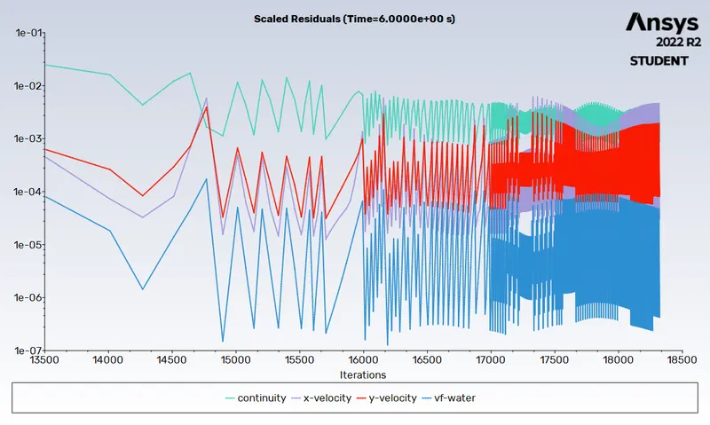
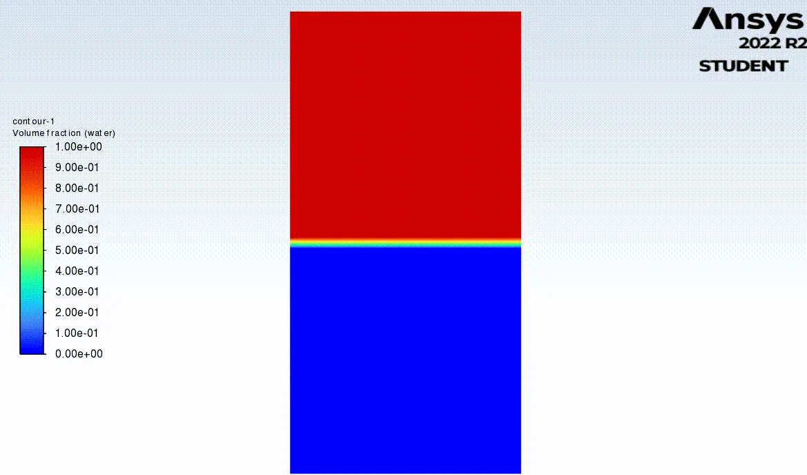
Now, we'll run the simulation with a Timestep size (s) of 0.005 with enough time steps until instability is resolved, or until stability in the domain is attained. Finally, the domain's top will be filled with air, while the bottom will be filled with water. Thus, the "Case 1" instability simulation is completed.

The 'Playback' tool will save the animation of the entire simulation in the fluent directory. As we don't need any additional data other than the simulation animations to draw conclusions, this will be regarded as post-processing.

Note: If stability isn't achieved in the simulation, keep adding more time steps after each calculation, as needed.

Case 2:

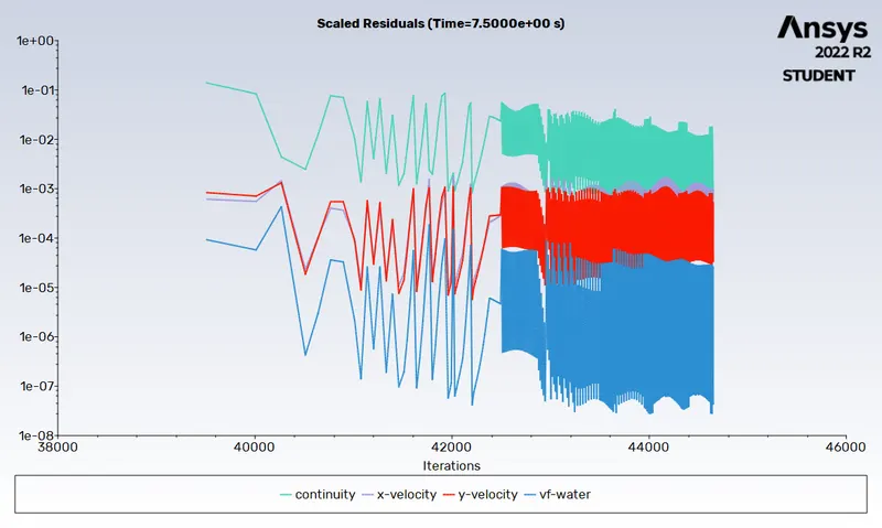
We will run the simulation with the timestep size (s) as 0.001 with a sufficient number of time steps until stability is achieved.

Case 3:

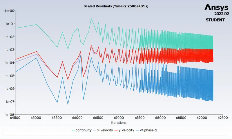
In this case, as we need to add new material, we will simply change the properties of air as - Density = `400 (kg) / m^3` & Viscosity = `0.001 (kg) / (mcdot s)` - and perform the simulation with timestep size (s) as 0.001 with increasing the number of timesteps if required.

RESULTS -

• Comparing simulation time with the help of 'Scaled Residual' plots -

The density difference between the two fluids was quite large in the first two cases, but it was much relatively small in the third. Since the first case used a coarse mesh, less time was needed for simulation. Whereas a finer mesh was created in the second case compared to case 1, the simulation took much longer. Case 3 required significantly more time than the first two cases because a finer mesh with a smaller density difference was used.

Cases	Scaled Residual Plots
Case 1
Case 2
Case 3

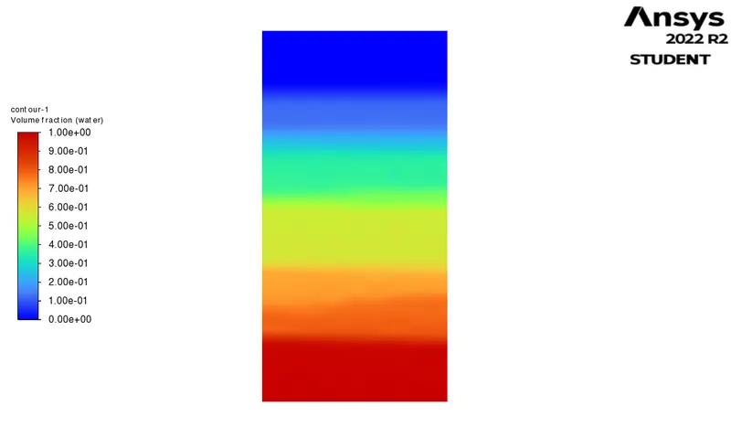
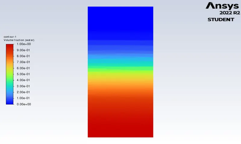
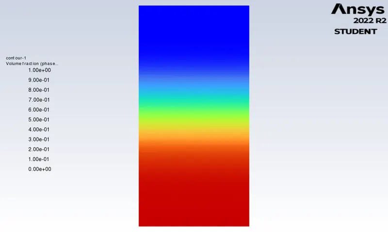
• Comparing results with the help of 'Volume Fraction Contour' plots -

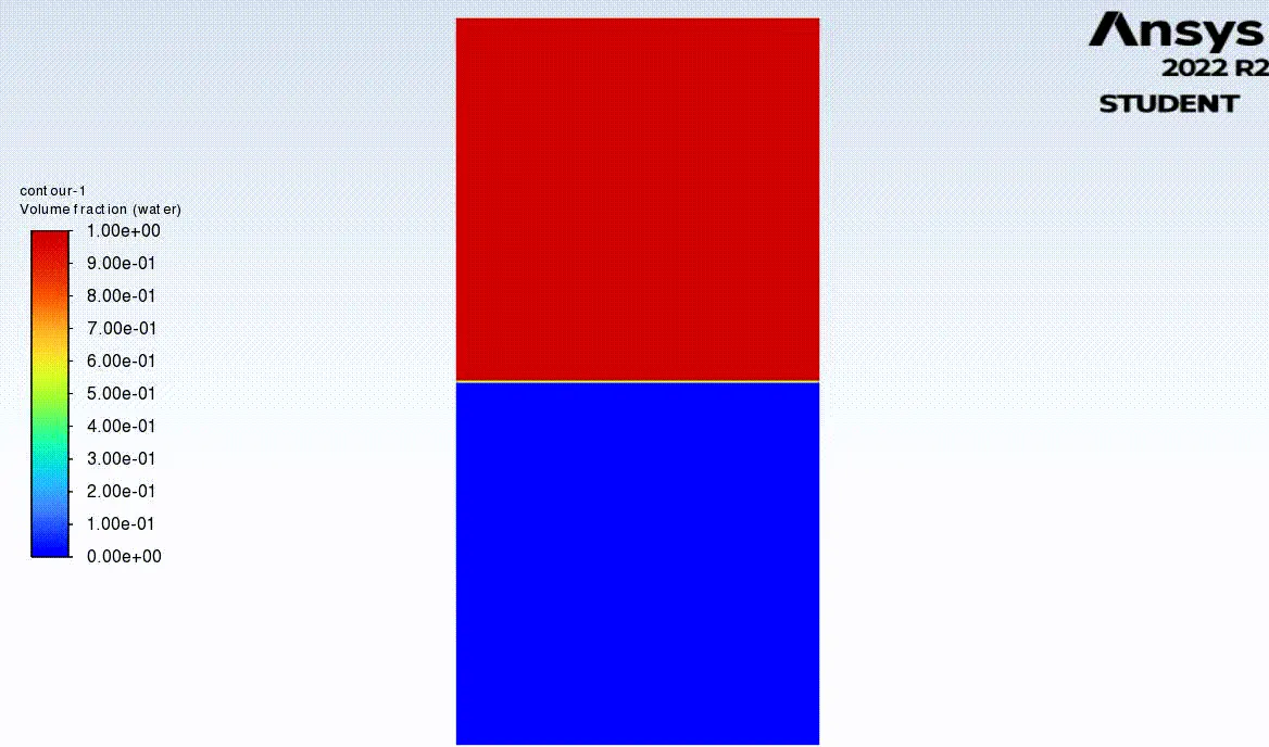
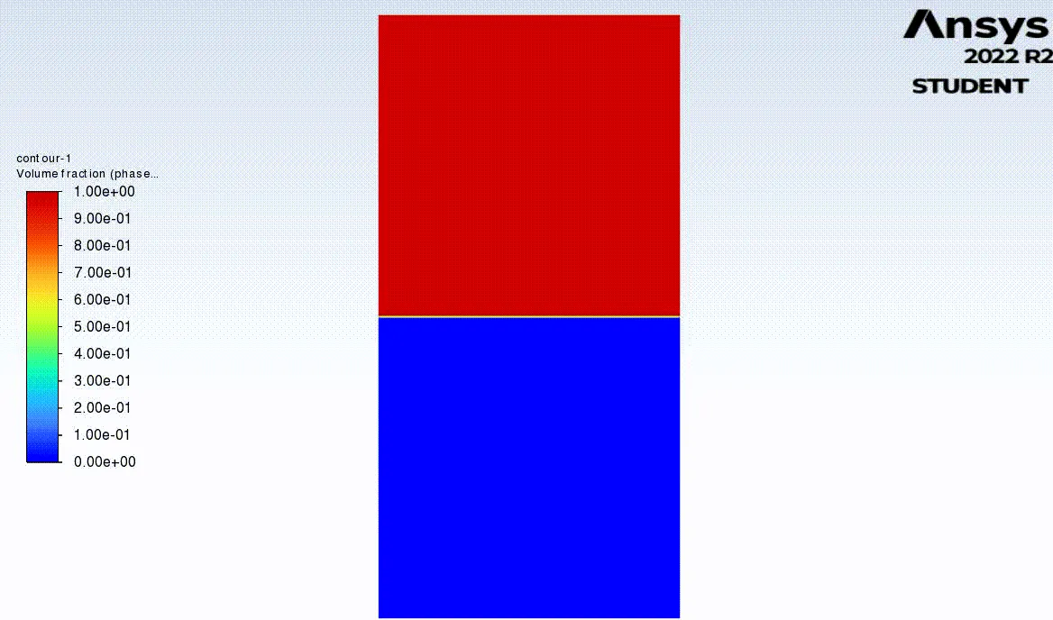
As the mesh size is decreased we get more defined results.

Cases	Volume Fraction Contour Plots
Case 1
Case 2
Case 3

• Calculating Atwood Number:

The Atwood number, A, is defined as the difference between the fluid densities divided by their sum.

For Cases 1 & 2 -

Let, density of water (`rho_1`) = 998.2 kg/`m^3` & density of air (`rho_2`) = 1.225 kg/`m^3`

`A = frac{rho_1-rho_2}{rho_1+rho_2} = frac{998.2-1.225}{998.2+1.225} = frac{996.975}{999.425} = 0.9975`

For Case 1	For Case 2

For Case 3 -

Let, density of water (`rho_1`) = 998.2 kg/`m^3` & density of user-defined material [air] (`rho_2`) = 400 kg/`m^3`

`A = frac{rho_1-rho_2}{rho_1+rho_2} = frac{998.2-400}{998.2+400} = frac{598.2}{1398.2} = 0.4278`

For Case 3

As mentioned earlier, for an Atwood number near zero, Rayleigh Taylor instability flows show as symmetric fingers of fluid, whereas for an Atwood number close to one, the much lighter fluid below the heavier fluid appears as larger bubble-like plumes.

During the instability simulations, the same correlation is found. In the first two cases, the lighter fluid (air) created bubble-like extensions before reaching the top. In the third case, even though, the atwood number was not close to zero, until the final stage of stability, the entire fluid domain, to some extent, appeared as finger projections.

Click here to see animations of all the three cases to have a better understanding of the aforementioned phenomena.

CONCLUSION -

1. It can be deduced that when there is a small density difference between fluids, a large amount of simulation time is needed to settle both fluids, and the opposite is true for fluids with a large density difference.

2. Fluids with much density difference have atwood number close to one, while fluids with small density difference possesses atwood number close to zero.

3. As the mesh quality increases, the results become more defined. That is, more clear and defined separation between the fluids is observed.

4. The fluids reach stability relatively early for simulations with atwood number close to one, but it takes longer for simulations with atwood number near zero to reach stability.
5. Since transient simulation is a time-marching solution and requires greater accuracy, it is the optimal configuration for computing Rayleigh Taylor Instability problem.

REFERENCES -

• Study of Rayleigh Taylor Instability with the help of CFD simulation
• Ansys Fluent User Guide
• Ansys Fluent Theory Guide

Thus, transient state simulations for Rayleigh Taylor Instability were performed, and inferences were derived based on the outcomes.