Week 5 - Rayleigh Taylor Instability
THEORY
Consider 2 immiscible fluids of varying density ρ1 & ρ2, such that ρ1≠ρ2. The interface line seperates 2 fluid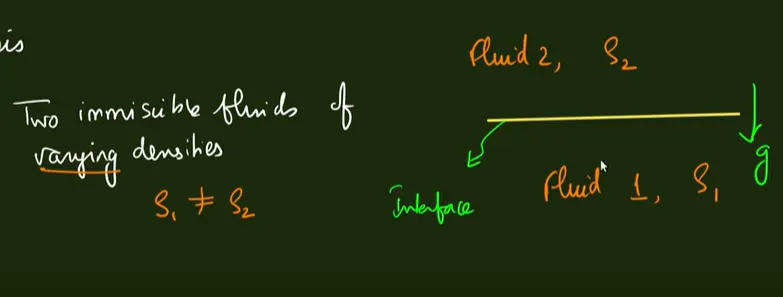
If ρ1>ρ2, the system is stable.
If ρ1<ρ2, this is unstable configuration,
then the dense fluid will overturn and the heavier fluid will come down and the lighter fluid will go up this overturning instability due to buoyancy or gravity is called the rayleigh tailor instability
Case setup
GEOMETRY
- Open SpaceClaim and draw a 20X20 mm square and select pull tool to make this a surface.
- Do the same thing above this square.
Geometry Prepared is shown below with dimensions.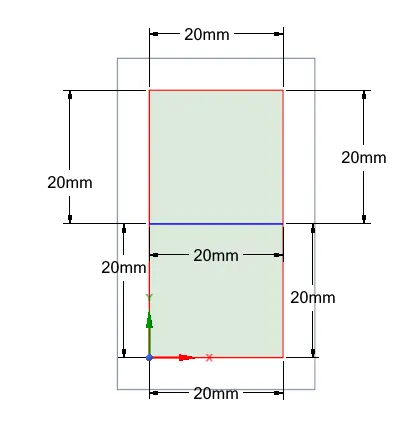
- Share topology.
Give the name as water for top face and air for bottom face
MESHING
- Create a baseline mesh of element size 0.5mm.
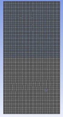
- Further refine the meshes by changing the element size.
mesh element size 0.3mm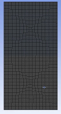
mesh element size 0.2mm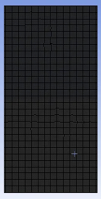
SETUP
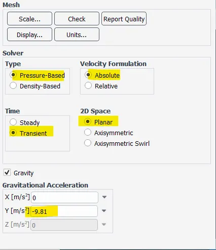
- General setup
- solver type: pressure based
- velocity formulation: absolute
- Time: transient
- 2D space: Planer
- gravity enabled with `y=-9.81m/s^2`
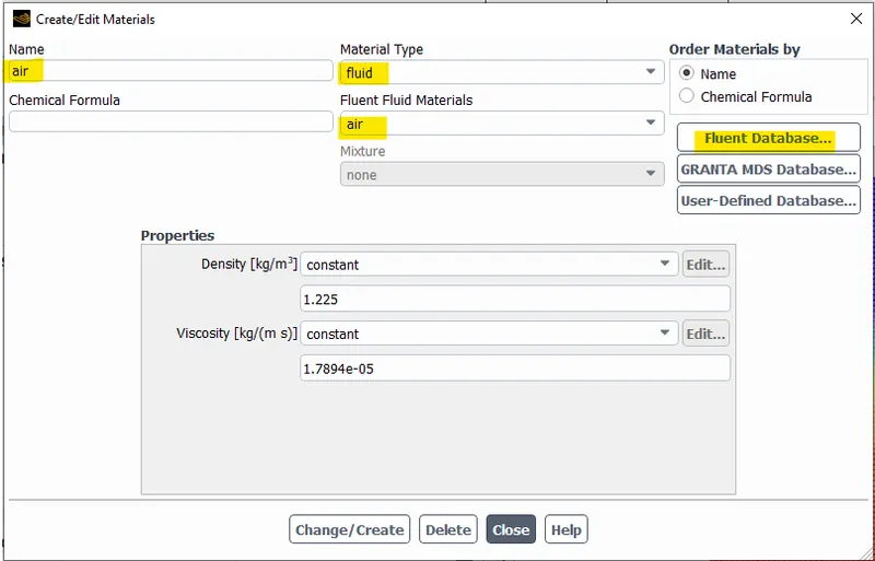
- Add materials
- fluid: air
- fluid" water liquid
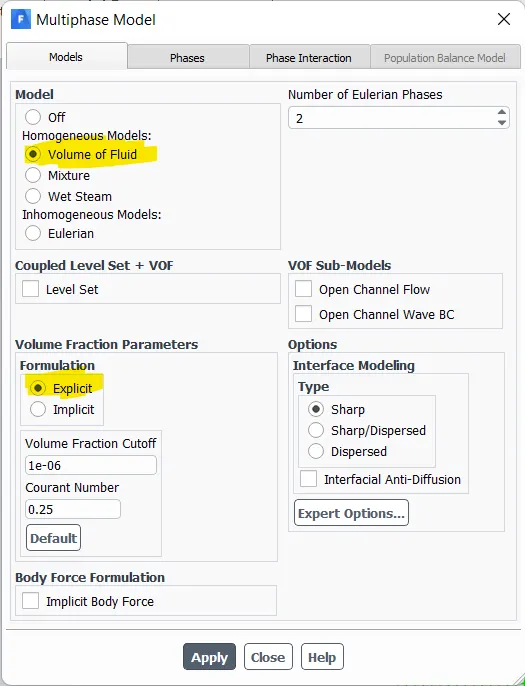
- Multiphase
- set multiphase model to Volume of fluid and explicit formulation.
- Rename phases by selecting the correct material for the phase.
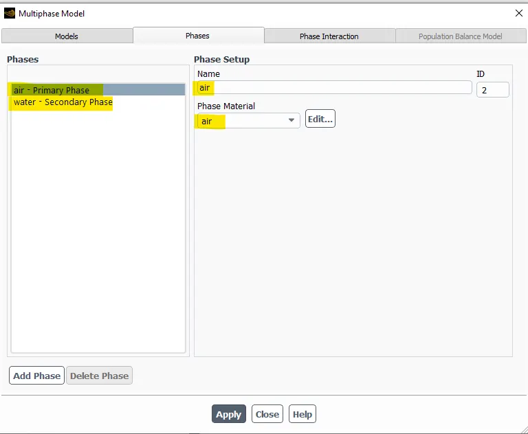
- set multiphase model to Volume of fluid and explicit formulation.
- Initialization
- initialize the setup with standard initialization.
- Patching
- After standard initialization, we need to patch both the respective materials, where we provide a volume fraction value of 1 for the water and 0 for the air and user defined material.
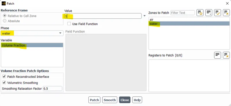
- After standard initialization, we need to patch both the respective materials, where we provide a volume fraction value of 1 for the water and 0 for the air and user defined material.
- contour creation.
- Create a contour for the reighleigh taylor method.
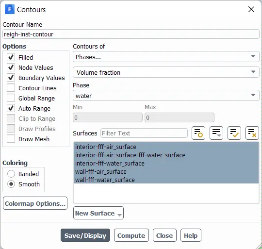
- Create a contour for the reighleigh taylor method.
- Animation creation
- create a animation for the result.
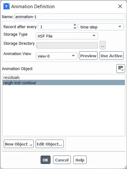
- create a animation for the result.
RESULTS
1) for baseline mesh (0.5mm)
Explicit method
The time step size is used for this simulation is 0.001 and it is fixed timestep. Flow time = 3 sec.No of time step = 3000.
The video is attached below as mesh5airwater.wmv
Google drive https://drive.google.com/file/d/1S7S19VXiUpYuD0ce_ZOhb4BSpV-aGwen/view?usp=sharing
2) for refined mesh (0.3mm)
a)Explicit method
The Courant number is set to 0.6. Here I used adaptive time step
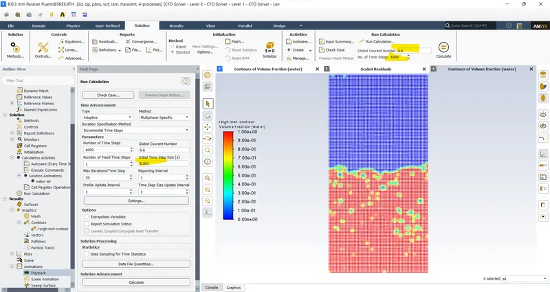
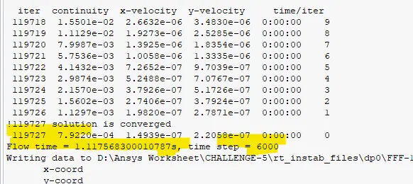
The flow time, time step and iteration are shown below
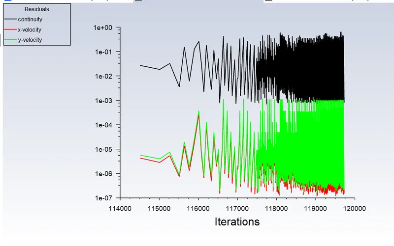
Scaled Residual
The animation frames are recorded at every 0.05 sec of flow time
The video is attached below as water-air03.mp4
Google drive https://drive.google.com/file/d/1QwgXqjPsRKS0FzjjkVzDmS2IHcOkxd9q/view?usp=sharing
We can view in slow motion by changing the settings of the media player.
It take more time(nearly 3 sec) to get fully settle, due to the presence of confining wall.
I stopped the simulation at flow time of 1.117 sec in order to save time.
b) Implicit method
The time step size=0.005, No of time steps=1000
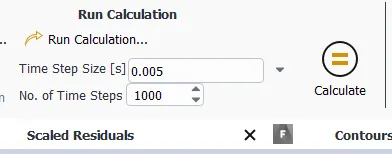
The flow time is 5 sec. The animations are recorded for every 0.05 seconds of flow time
The video is attached below as water-air_imp03.mp4
Google drive https://drive.google.com/file/d/1nmV9OWmaXcJ8vPbVMgPLRKyHn7RUN5XF/view?usp=sharing
3) for mesh (0.2 mm)
Implicit method
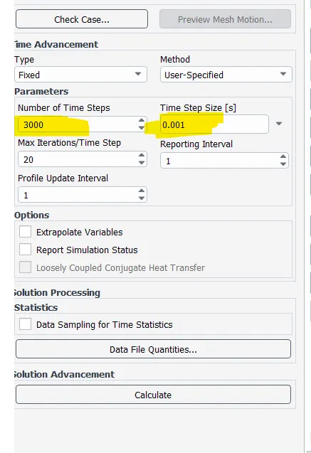
The solution is run for 3 sec.
The video file is attached below water-air_02_imp.mp4
Google drive https://drive.google.com/file/d/15sTDsQamESgQSCUTxg7yBYvg7YiP3VY6/view?usp=sharing
Atwood number
At=(ρ_water - ρ_air) /(ρ_water + ρ_air)
At = (998.2 - 1.225)/(998.2 + 1.225) = 0.997548
CONCLUSION
1) The implicit method takes more time to get the solution when the mesh is refined(0.2 mm) and the time step is reduced(0.001 sec).
Reducing the time step will give most accurate result
2) Explicit method is giving good result when the mesh size is larger(0.5 mm) and with the time step size of 0.001 sec. The air bubbles in water and liquid droplets in air can be clearly visible in explicit method during simulation. So, it is the best method to view the intermediate results.
3) The air-water is a long wave and k X lc->0. So, the perturbation is higher and it increases exponentially. Also Atwood number is close to 1 for this case.
where k is the wave number
lc is the capilary length
Here, the growth rate increases exponentially and it is a case of large wavelength. The presence of walls will affect the growth rate. That's why it is taking more time to come to stable position. If there is no wall on top, it comes to equilibrium position faster and the perturbation growth rate is higher.
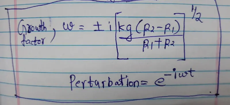
Here, the growth factor is purely imaginary. Then the perturbation term will be real term and it increases exponentially as shown in equation below.
The relation between growth factor and perturbation term for long waves is shown below.
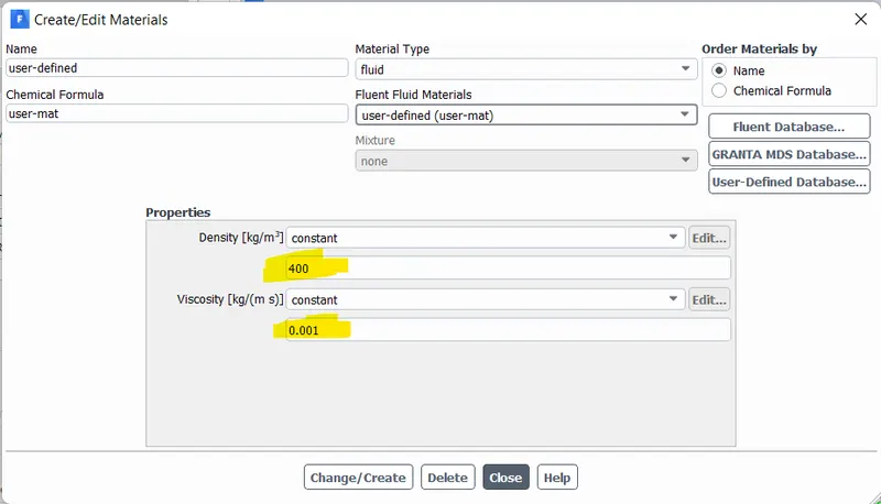
Run one more simulation with water and user-defined material(density = 400 kg/m3, viscosity = 0.001 kg/m-s) for refined mesh.
I m using implicit method with mesh size 0.3 mm.
If the Surface force is taken into account, this give rise to the chance of capilary waves such that the denser fluid will remain on top of the lighter fluid and it creates short capilary waves such that it maintains a stable equilibrium. Here, mostly the denser fluid will take more time to settle down.
In case of capilary waves, the growth factor is real and the perturbation term is imaginary and it comes in denominator. This gave rise to short capilary waves.
The relation between growth factor and perturbation term for capilary waves is shown below.
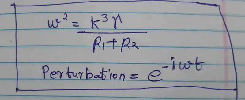
Where γ(Gamma) is the Surface tension term. k is the wave number.
User material proof
Implicit method
Mesh = 0.3 mm, time step size = 0.005 sec.
Flow time = 6 sec
The video is attached below as water-user_imp_03.mp4
Google drive https://drive.google.com/file/d/14DA8aOXn7r3UDw3XUp5j-RKeB3d_BtPX/view?usp=sharing
FINAL CONCLUSION
1) The air-water phase takes nearly 2-3 sec to settle down, but user material-water phase takes 5-6 sec to completely settle down
2) The explicit method is used for cases that run for a short duration of time(as per Ansys user manual video). The intermediate results and final results are clearly distinguishable in case of explicit method. In implicit method, we get a value between 0-1 at some cells which is identified from the colour of the cells, but in explicit the colour is easily distinguishable between blue and red.
3) When I done simulation with mesh size 0.5 mm with explicit type, I observed the liquid droplets in air medium and air bubbles in liquid medium respectively. It partially behaved like Dispersed Continous phase interactions. But the system is mostly Continous-Continous phase interactions.
Define the Atwood Number. Find out the Atwood number for both the cases and explain how the variation in Atwood number in the above two cases affects the behavior of the instability.
It is a non dimensional number that is used to study hydrodynamic instability in density stratified flows.
At=(ρ1 - ρ2) /(ρ1 + ρ2)
where,
ρ1 is density of heavier fluid
ρ2 is density of lighter fluid
For air-water interface
At=(ρ_water - ρ_air) /(ρ_water + ρ_air)
At = (998.2 - 1.225)/(998.2 + 1.225) = 0.997548
Flow time to stabilise = 2-3 sec
For user-defined - water interface
At=(ρ_water - ρ_user) /(ρ_water - ρ_user)
At = (998.2 - 400)/(998.2 + 400) = 0.42783
Flow time to stabilise = 5-6 sec
When the Atwood number decreases it takes more time to stabilise.
Actually it is not the Atwood number determines the stability of the system.
Stability is determined by the growth factor ω, and then it is put in the equation for perturbance(growth rate) as exp(-iωt).
As mentioned above, if a heavier fluid is on top of the lighter fluid, it can also be in stable equilibrium by making short capilary waves. The heavier fluid need not necessarily come down. It depends on surface tension between the fluids and density difference between the fluids. In this case, the growth factor ω is purely real, and the perturbance(growth rate) is purely imaginary. This gave rise to small capilary waves.
In our challenge, there are walls on top and side where the 2 fluids are enclosed. The perturbance(growth rate) is affected by walls in case on longer wavelength cases. For air-water, it is a case of sufficiently longer wavelength. Due to the presence of walls, it takes nearly 2-3 seconds to settle. If the top and side walls are at infinite distance, the air-water will settle suddenly.
For case 2, if the surface tension force is taken into account, it might be a chance of small capilary waves. But in our challenge, it is a large wave, but not larger than air-water.
What are some practical CFD models that have been based on the mathematical analysis of Rayleigh Taylor waves? In your own words, explain how these mathematical models have been adapted for CFD calculations.
We used Eulerian multi phase model.
It is of 2 types
a) Dispersed-Continous phase interactions
b) Continous-Continous phase interactions
The examples of Dispersed-Continous phase interactions are shown below. Dispersed phase can be particles(solids), droplets(liquids) and bubbles(air).
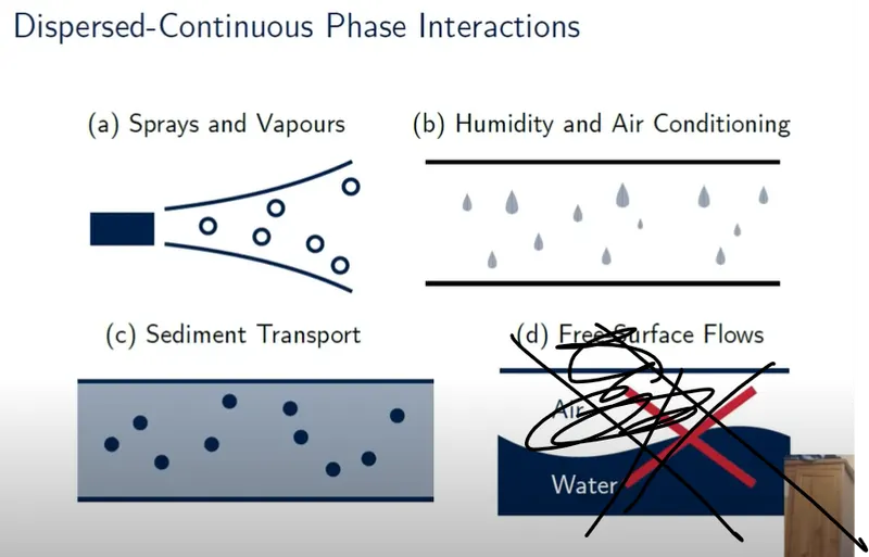
The continous-continous phase interaction is shown below. They are immiscible with each other.
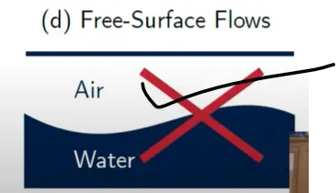
In our challenge, it is an example for continous continous phase interaction.
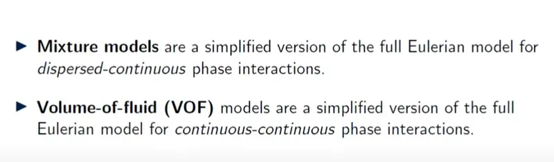
The practical models that can be used for mathematical analysis of Rayleigh Taylor waves are Mixture models and Volume of Fluid(VOF) models.
In our challenge, we used VOF model as we want to see the continous-continous phase interactions.
The Mixture models and Volume of Fluid(VOF) models are explained below
Also, explain why a steady-state approach might not be suitable for these types of simulation
The Rayleigh Taylor instability is a time based instant. If a heavy fluid is on top of the light fluid, it comes to bottom due to gravity. It is a time based event. Any freely falling body is a transient condition. After it fell down, it is a steady state.
Any transient state may or may not be a steady state after the passage of time. If the heavy fluid is on top of the light fluid if the heavy fluid does not come down and it produces capilary waves, it is a condition of steady state.
Observe the differences in the animation and explain the effect of mesh size on simulation
As the mesh size increases, the simulation time increases for implicit and explicit cases