Week 5 - Rayleigh Taylor Instability

Aim- To conduct the Rayleigh instability CFD simulation and understand the phenomenon.

Objective-

• To understand the practical CFD models that are based on the mathematical analysis of Rayleigh Taylor waves.
• Perform the Rayleigh Taylor instability simulation with two different types of mesh element constraints and compare the result between both.

Theory-

• Rayleigh Taylor's stability states that it is an interpenetration of the materials that occur when a light fluid pusses the heavy fluid. It is a dynamic process where the two fluids seek to reduce their combined potential energy. Initially, the system is in a state of hydrostatic equilibrium in which the heavier fluid(water) sits on top of the lighter fluid(air) in a constant gravitational field. It develops the initial perturbations and progresses from a linear growth phase eventually developing plumes flowing upwards and spikes flowing downwards.
• Practical CFD models
• SPH Method(smoother particles Hydrodynamics)- It is a computational method used for simulating the mechanics of a continuum media, such as solid mechanics and fluid flow. Smoothed particle hydrodynamics is being increasingly used to model fluid motion as well. This is due to several benefits over traditional grid-based techniques. First SPH guarantees the conservation of mass without extra computation because the particles themselves represent mass. SPH computes pressure from weighted contributions of neighbouring particles rather than by solving linear systems of equations. Unlike the grid-based techniques which must track fluid boundaries, the SPH creates a free surface for two-phase interacting fluid fluids since the particle represent a denser fluid and space represent a lighter fluid.
• Single Fluid Model- The approach used for the analysis of two-phase flows is a mixture model i.e the individual fluid phases are assumed to behave as a flowing mixture described in terms of the mixture properties. The applied single fluid model is a five-equation model consisting of energy, mass and momentum equations for a vapour/liquid mixture, and two equations describing the formation and growth of the liquid phases.
• Two-Fluid Model- In the two-fluid model, separate sets of the governing equation from the vapour and the liquid phase have been used. The interactions between the droplets and the heat exchange between the liquid phase and the solid boundary are not modelled here as well. The velocity slip between the vapour and the liquid phase in this model is considered.
• Turbulence model- A turbulence model is needed to predict the average mixing behaviour that is on the average one- or two- dimensional. The approach to the construction of the title turbulence model is guided by experimental behaviour. the equation governing turbulent flow can only be solved directly for simple cases of flow.

Geometry-

• We have to make a 2d model for the analysis and a study of Rayleigh Taylor instability. For that, we will go with two rectangular faces above each other as a replication or simulate important entities for this study. i.e; water, air.
• 20mm*20mm will be the dimensions of the two rectangular faces.

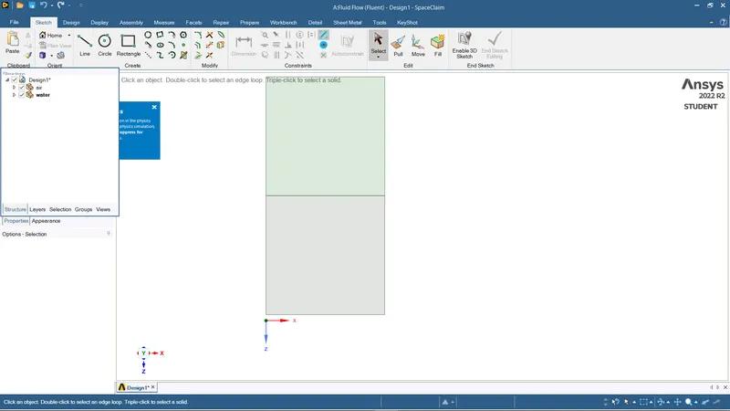
• Because it is a 2d simulation we will use a pulling tool to give base surface extensions to the faces.

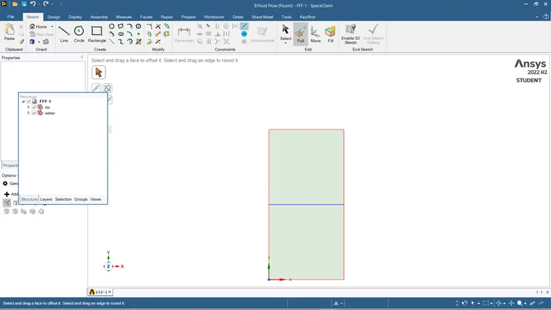
• For that just click on the pull tool and select the entity, click Esc and space claim will automatically apply the surfaces.

Mesh-

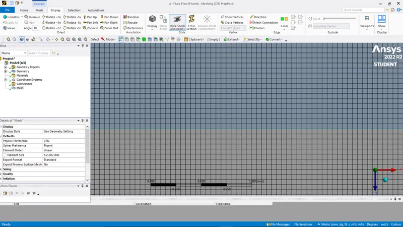
We don’t need to do or give any meshing constraints because it is a 2d geometry.

• While meshing we go with the element size of 0.5mm.

Setup-

• For this simulation we go with the transient simulation type and with the pressure-based solver and velocity formulation will be an absolute and viscous model as laminar.

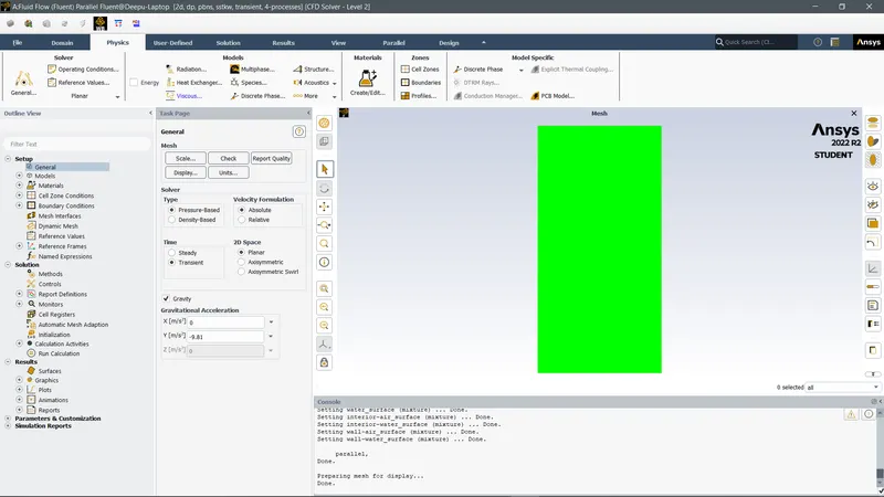
values

• Time- transient
• Velocity formulation- absolute
• Solver- pressure-based solver
• Gravity- x=0,y=-9.81(because the y direction is considered as downward),z=0
• The next step would be Setting up the physics
• Viscous model- laminar flow
• Enable multiphase method

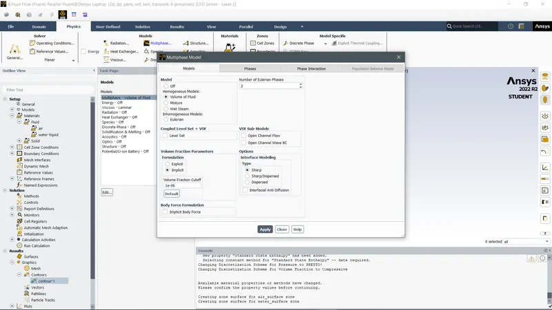
• Homogenous model- the volume of fluid
• Formulation – implicit
• Number of eulerian phases- 2

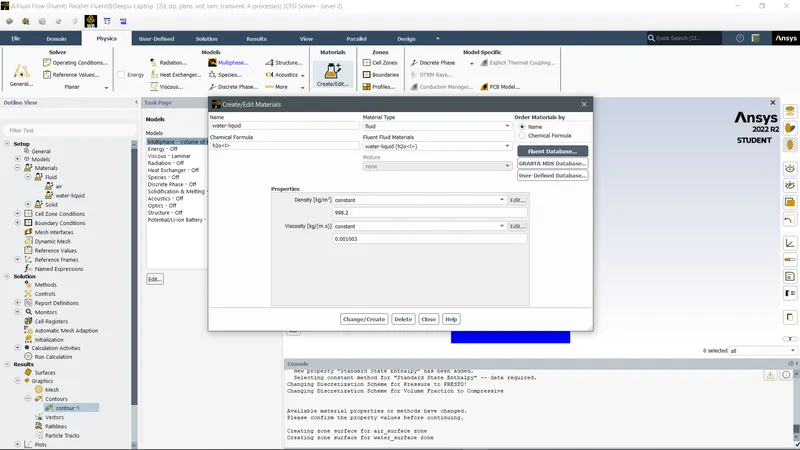
• Materials create/edit
• Fluid -fluent database-search for water- copy-close
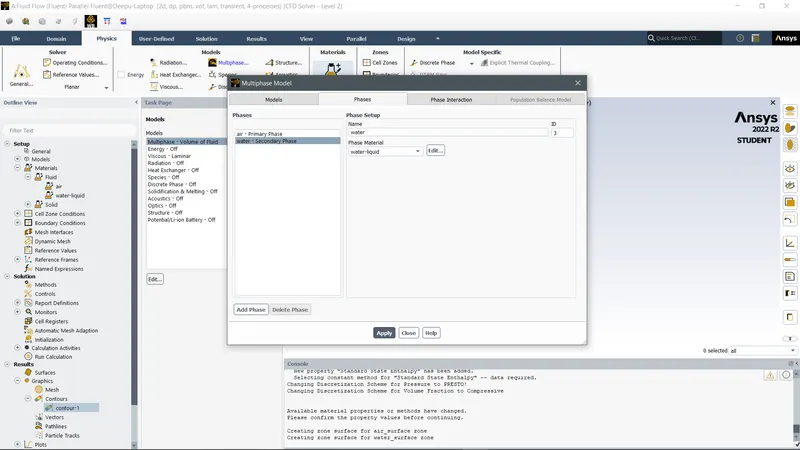
• Phases rename phase 1 air as air and phase 2 water as water.

• We need to ensure that the air is at the top and the water is at the bottom position. For that, we have to patch the entries. For patching go to patch and select phase as water and variable- volume function, value =1 as the water should be on top and then for Air- select phase air and value-0 as the air should be on the bottom.

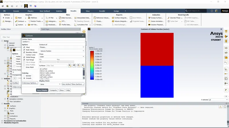
• To check whether the selection is correct we go with the CONTOUR option
• Contour- new select contours of phases and then select water and- click display.
• 0 shows the air and water shows 1

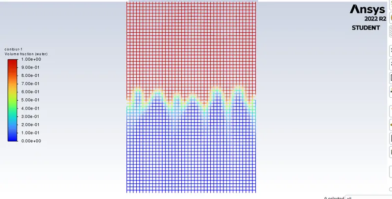
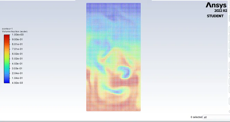
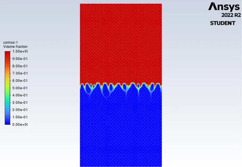
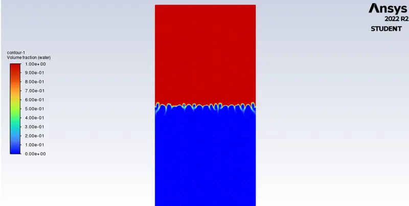
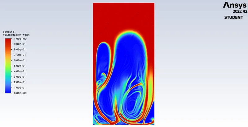
Case-1

Mesh element size-0.5mm

Time steps size-0.01

No of time steps- 100

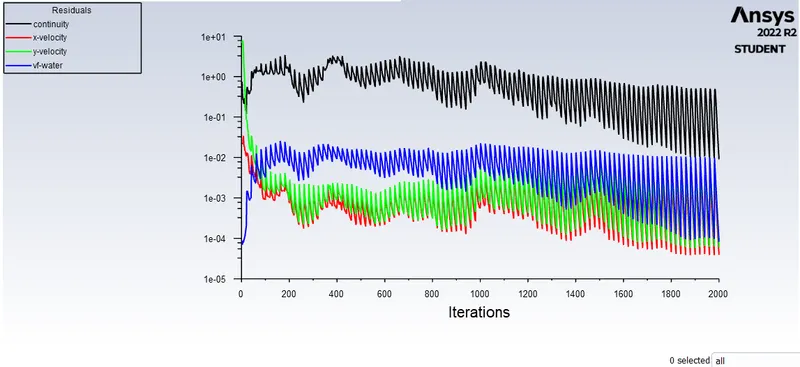
Simple Scheme Solution

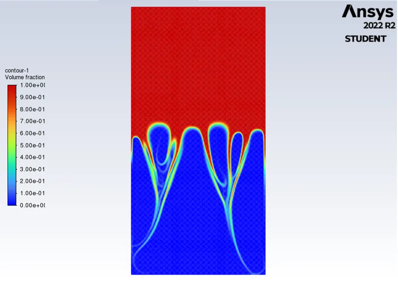
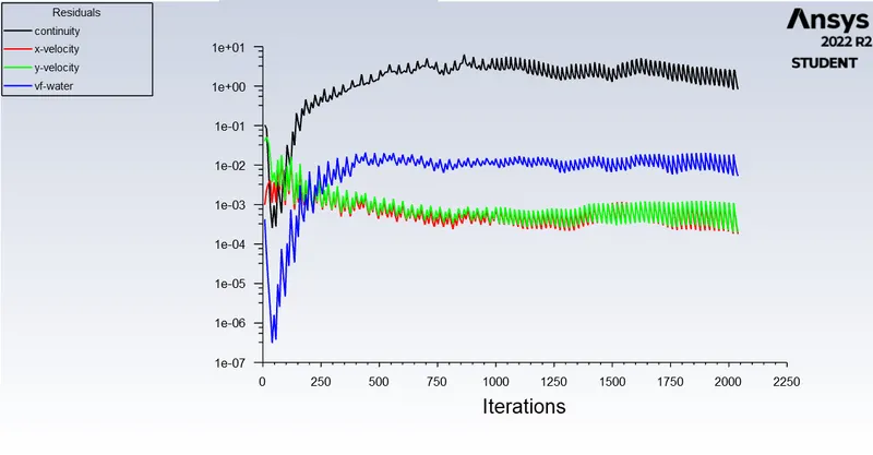
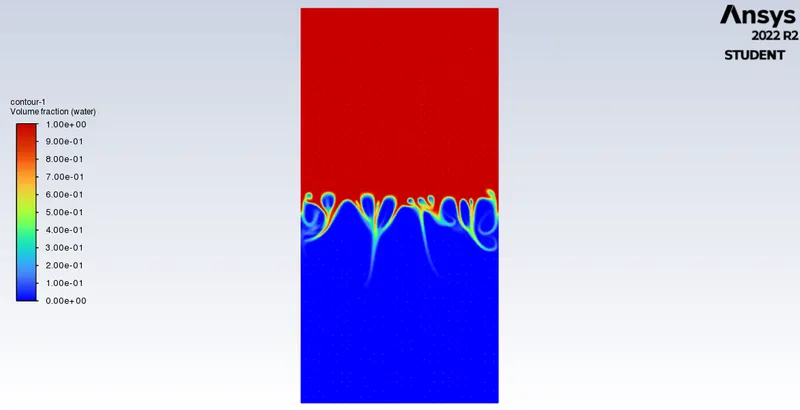
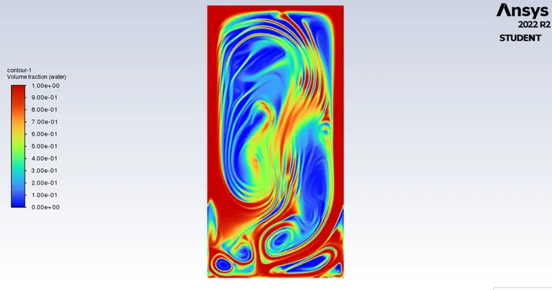
Case-2

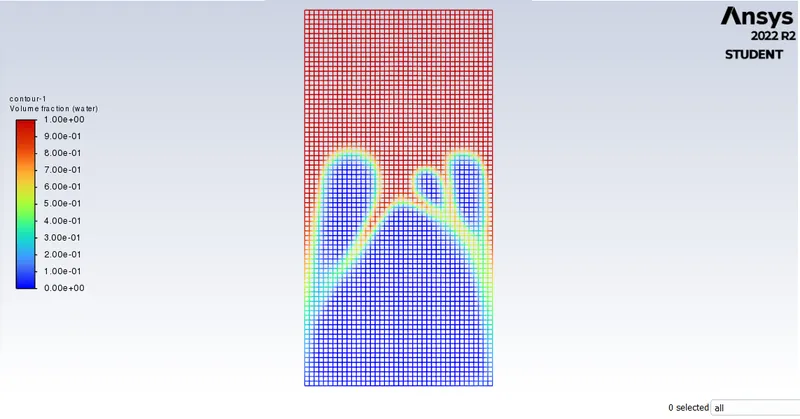
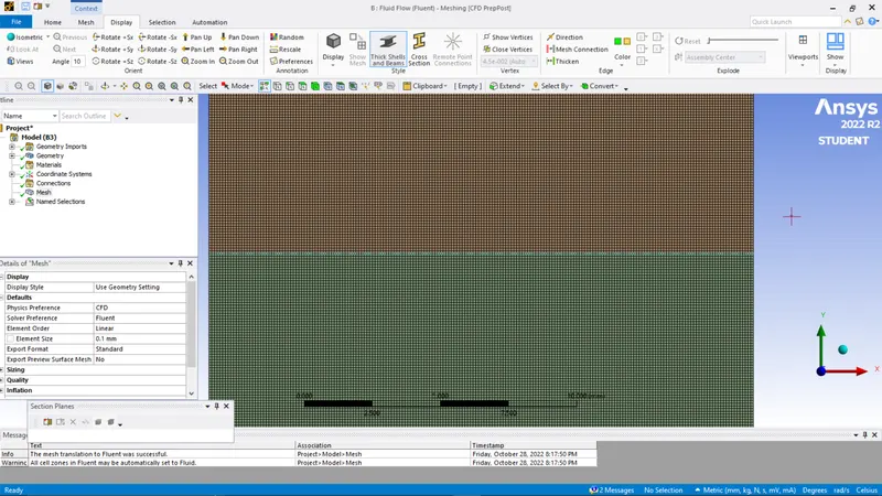
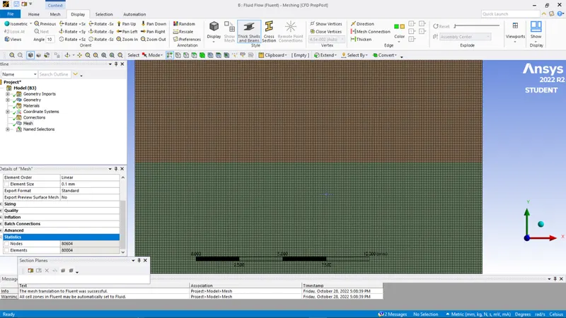
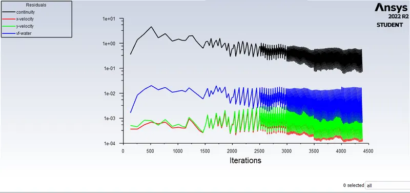
Mesh element size-0.1mm

Time steps size-0.005

No of time steps- 1500

Coupled Scheme Solution

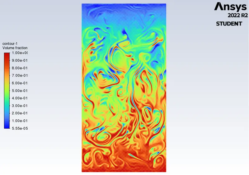
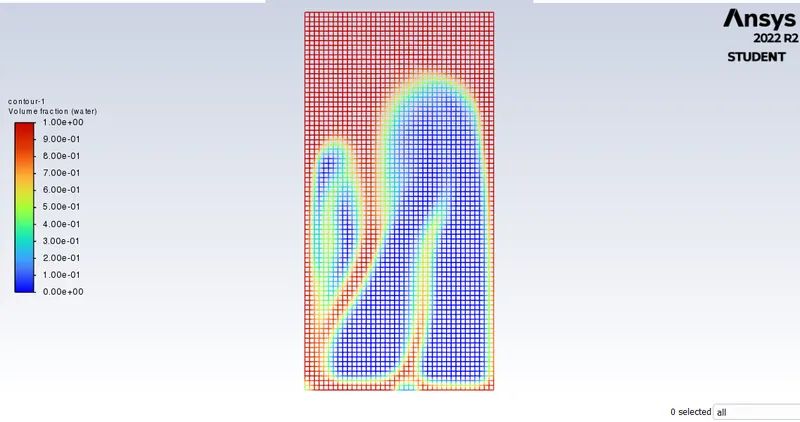
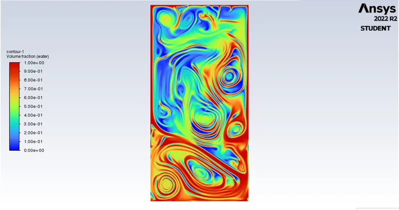
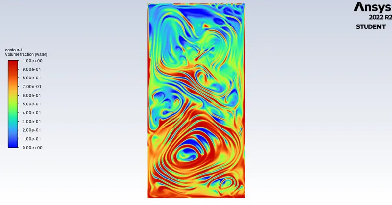
Case-3

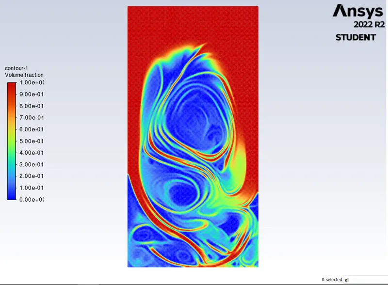
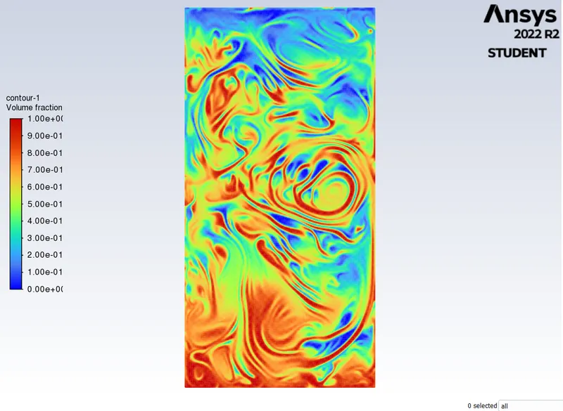
The properties of the water are changed-

Density- 400 kg/m^3

viscosity- 0.001kg/m-s

Mesh element size-0.1mm

Time steps size-0.005

No of time steps- 1500

Coupled Scheme Solution

Atwood Number-

Atwood number is a dimensionless fluid in the fluid dynamics used in the study of hydrodynamics instability in density-stratified flows. it is a dimensionless density ratio defined as

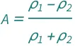
where P1= density of the heavier fluid

P2= density of the lighter fluid

In Rayleigh Taylor instability the penetration distance of heavier fluid bubbles into the lighter fluid is the function of the acceleration time scale.

Agt^2

where g= gravitational acceleration , t= time

P1=997

P2= 1.225

A=997-1.225/997+1.225 = 0.99754

The behaviour of RTI stability on the variation of Atwood Number.

RTI evolves in three different stages- linear stability, mushroom head, bubble formation, long term evolution due to merging and mixing. For low Atwood numbers, bubble, and mushroom head shape is relatively symmetrical, and the disturbances or perturbations are linear for a larger time. In contrast, for large Atwood number, bubble and mushroom head shape is less symmetrical, also it occurs very rapidly at an accelerating rate which leads to a nonlinear growth rate.

Conclusion-

• By analysing the above cases we found that the finer mesh gives better instability results than coarse mesh, but the finer mesh needs more computational power and is more time-consuming.
• In this calculation Transient approach is preferred approach over the steady state approach because the simulation needs to capture the unpredictable motion of fluid with respect to time.
• The Atwood number validates the CFD simulation as it is observed. In the case of water and air mixing, bubble formulation takes place.