Week 5 - Rayleigh Taylor Instability

Objective: To perform Rayleigh-Taylor instability study using CFD simulation.

Introduction:

Experiments performed to study the physics of certain phenomenon are costly and time-consuming. Numerical simulation is developed and used to reduce the time needed to study the nature and physics involved in the system of interest. This method indeed provides results very fast compared to experiments but they lack a bit in terms of accuracy. If the experiments take a month to produce results, simulation might take a day and give us results 90% accurate. In the fast-paced world, where developing various solutions require faster results, engineers make a delicate balance between the accuracy and time taken as necessary.

All fluid flows are governed by three equations -Continuity, momentum and energy equations. We need to solve these equations for the given conditions to understand the fluid behavior. Computers are incapable of solving these equations in their integral and differential forms. So, we can divide our geometry into many tiny elements (called mesh) and modify the governing equations into difference equations that can be solved by the computer. We apply these difference equations for all the elements in the geometry and generate an approximate solution. It is hence necessary to validate these results against the experimental data.

The number of difference equations, for a given problem varies with the nature of physics involved. We typically solve a finite number of equations at all the elements. These equations are grouped together, called a turbulence model. A lot of work has been put into developing and improving the turbulence models and the work still goes on today. Examples of turbulence models are S-A, k-epsilon, k-omega etc.

Theory:

In fluid dynamics, hydrodynamic stability is the field which analyses the stability and the onset of instability of fluid flows. There are many kinds of instabilities across various fields. A few of them are:

Plateau–Rayleigh instability:

A falling stream of fluid breaks up into smaller packets with the same volume but less surface area. This phenomenon occurs due to surface tension of the fluid and tendency of the liquid to maintain minimum surface area. This is observed when water falls from a faucet.

Kelvin–Helmholtz instability:

When there is velocity shear in a single continuous fluid or a velocity difference across the interface between two fluids. Vortex formation occurs along the edge of a free axisymmetric jet due to shear force between the high velocity jet and the stagnant surrounding air.

Richtmyer–Meshkov instability:

When two fluids of different density are impulsively accelerated. Normally, by the passage of a shock wave. This instability can be considered the impulsive-acceleration limit of the Rayleigh–Taylor instability. Supersonic combustion in a Scramjet is enhanced by the breakup of the fuel into finer droplets due to this effect.

Saffman–Taylor instability:

It occurs when a less viscous fluid is injected, displacing a more viscous fluid. This is also known as viscous fingering. This situation is most often encountered during drainage processes through media such as soils.

Rayleigh-Taylor instability:

This is the subset of Saffman-Taylor instability and it occurs when driven by gravity (without injection) if the interface is horizontal and separates two fluids of different densities, the heavier one being above the other, known as the Rayleigh-Taylor instability. Examples include the behavior of water suspended above oil subjected to gravity of Earth, mushroom clouds like those from volcanic eruptions, atmospheric nuclear explosions and supernova explosions.

Modelling approaches for multi-phase flows:

There are different ways in which we approach multi-phase physics like:

Euler-Lagrange approach:

In this approach, particles are tracked on the level of a single particle where particle refers to either a solid particle or a gas/fluid bubble/droplet. As this modelling approach resolves information on the level of a single particle it is quite computationally expensive and therefore Euler-Lagrange modelling is suitable.

Euler-Euler approach:

In Euler-Euler models all phases are treated as continuous. The phases are treated separately and one set of conservation equations are solved for each phase.

Volume of fluid approach:

The VOF method uses a phase indicator function, sometimes also called a colour function, to track the interface between two or more phases. The indicator function has value one or zero when a control volume is entirely filled with one of the phases and a value between one and zero if an interface is present in the control volume. Hence, the phase indicator function has the properties of volume fraction.

Courant number:

The Courant number is a dimensionless value representing the time a particle stays in one cell of the mesh. It must be below 1 and should ideally be below 0.7. If the Courant number exceeds 1, the time step is too large to see the particle in one cell, it “skips” the cell. If it is smaller than 0.7, the particle stays in the cell for at least two time steps.

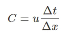
Where u is velocity magnitude,

Δt is time step size,

Δx is the length between mesh elements.

When the Courant number exceeds the value of 1, instabilities are amplified throughout the domain and may cause divergence of the simulation.

Modelling in Ansys Fluent:

The work flow in Ansys Fluent would follow four steps:

1. Geometry creation.
2. Mesh generation.
3. Pre-processing settings and simulation.
4. Extracting results.

Geometry creation:

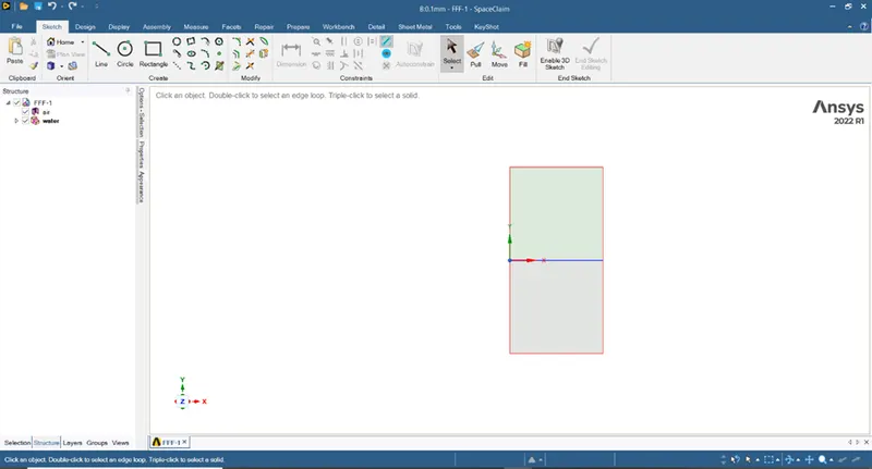
We create a new sketch to draw a rectangle of size 20mm x 20mm. We use Pull tool to create a surface. We repeat the same and create another rectangular surface over this surface.

We use Share option to ensure proper flow of fluid data in the geometry.

Mesh generation:

The geometry used for this study is simple and hence we can use structured quad elements for meshing. We would use two meshes of element size 0.5, 0.1mm.

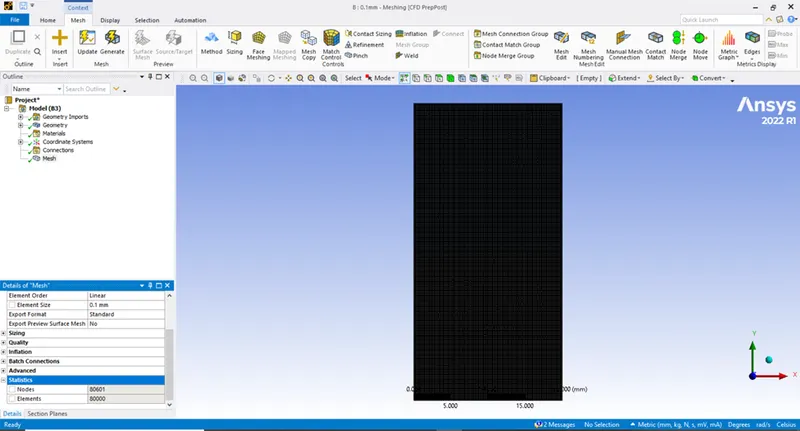
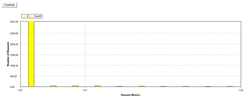
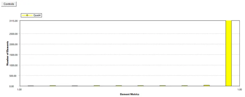
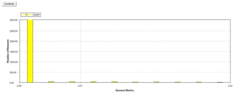
We need to look at the element quality and make sure it meets desired standards.

The best mesh would have aspect ratio, orthogonal quality close to 1 and skewness close to 0. The mesh we use conforms to the quality standards.

Pre-processing settings and Simulation:

We would proceed to Setup the conditions of the model. The process flow would be as follows:

1. Check the mesh in the solver.
2. Choose the turbulence model.
3. Create necessary materials and enable multi-phase model.
4. We initialize and patch the materials appropriately.
5. Create Volume fraction contour for water and create an animation.
6. Run the simulation for given number of time steps.

Extracting results:

We save the data for every time-step and create an animation file to observe the fluid physics and deformation of the interface.

Settings used for current simulation:

We used Pressure-based solver, absolute velocity formulation, transient state simulation.

We enabled gravity and used laminar model. We use air and water as the working media.

We would use Volume of Fluid model and Implicit formulation. In the Phases section, we would assign air and water to primary and secondary phases respectively.

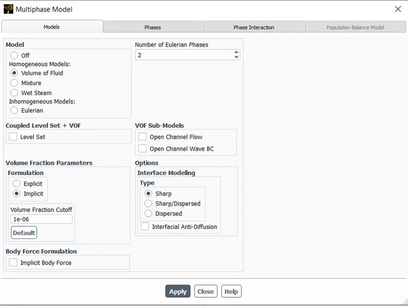
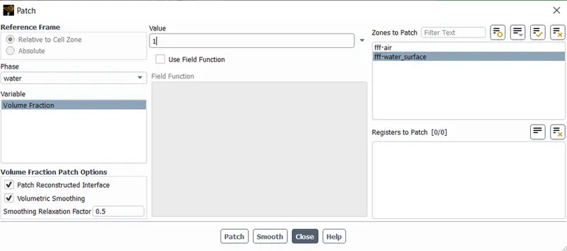
We can then initialize the solution and patch the phases to respective geometries. Since we don’t have inlet or outlet, we don’t see any assignment of values to the geometry. We assign the Volume Fraction of water phase as 1 and patch it. We assign the Volume Fraction of air phase as 0 and patch it.

Before we start the calculation, it is necessary to choose proper time step size to prevent diverging of the solution or having floating point exception error. We might get these errors due to large value of courant number which is a parameter used to study fluid instability.

Based on courant number criterion, we choose our time step size for the mesh size as mentioned in the following table.

We have run the calculation till the interface is observed to stabilize i.e., no notable change is observed in the fluids.

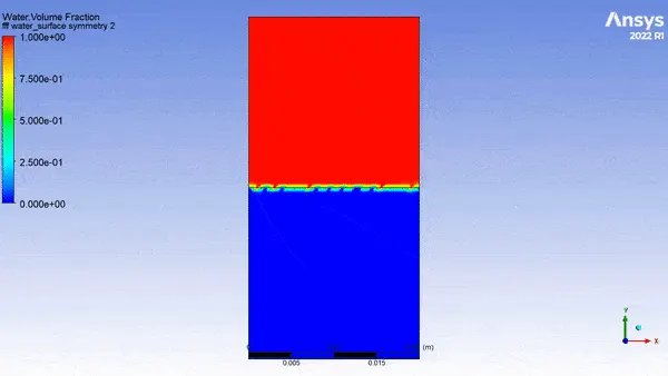
Case 1- 0.5mm – water, air:

We patched the top geometry with water and the bottom geometry with air. Due to gravity, water would end to fall down and fill the bottom geometry forcing the air upward.

Animation:

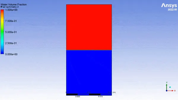
Case 2- 0.1mm – water, air:

We patched the top geometry with water and the bottom geometry with air. Due to gravity, water would end to fall down and fill the bottom geometry forcing the air upward.

Animation:

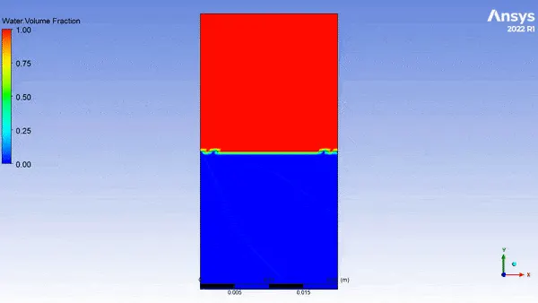
Case 3- 0.5mm – water, user-defined material:

We patched the top geometry with water and the bottom geometry with a new material. We assigned the properties as density = 400 kg/m³, viscosity = 0.001 kg/m-s. Due to gravity, water would end to fall down and fill the bottom geometry forcing the user-defined material upward.

Animation:

Atwood number:

It is a dimensionless number that is used to study hydrodynamic instabilities in density stratified flows.

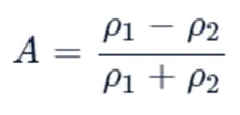
Where ρ1 is density of heavier fluid

ρ2 is density of lighter fluid

We calculate Atwood number for air-water instability study and water-user defined material instability study.

In Rayleigh–Taylor instability, the penetration distance of heavy fluid bubbles into the light fluid is a function of acceleration time scale, Agt².

Conclusion:

The Rayleigh- Taylor instability is studied for here cases and the animations are presented.

As the Atwood number is increased above 0.5, the consequence of the mixing asymmetry becomes more obvious: the two edges of the mixing layer develop into “spikes” on the light fluid side and “bubbles” on the heavy fluid side. For Atwood number below 0.5, the interface deforms slowly and mixing happens slower as well.

References:

1. Roberts, M. S. (2020). Fluid Instabilities and Transition to Turbulence. In K. Ghaedi, A. Alhusseny, A. Nasser, & N. Al-Zurf (Eds.), Computational Overview of Fluid Structure Interaction. IntechOpen.
2. https://en.wikipedia.org/
3. Saha, I. Study of Rayleigh Taylor Instability with the Help of CFD Simulation. Preprints 2020, 2020070385 (doi: 10.20944/preprints202007.0385.v1).
4. https://www.simscale.com/knowledge-base/what-is-a-courant-number/#:~:text=The%20Courant%20number%20is%20a,it%20%E2%80%9Cskips%E2%80%9D%20the%20cell.
5. https://publications.lib.chalmers.se/records/fulltext/182902/182902.pdf
6. https://www.lanl.gov/orgs/adtsc/publications/science_highlights_2010/9livescu.pdf