Week 5 - Rayleigh Taylor Instability

Aim -

1. What are some practical CFD models that have been based on the mathematical analysis of Rayleigh Taylor waves? In your own words, explain how these mathematical models have been adapted for CFD calculations.
2. Perform the Rayleigh Taylor instability simulation for 2 different mesh sizes with the base mesh being 0.5 mm. Compare the results by showing the animations( Attach them from your google drive). Observe the differences in the animation and explain the effect of mesh size on simulation. Also, explain why a steady-state approach might not be suitable for these types of simulation.[ Choose Air and Water for this simulation]
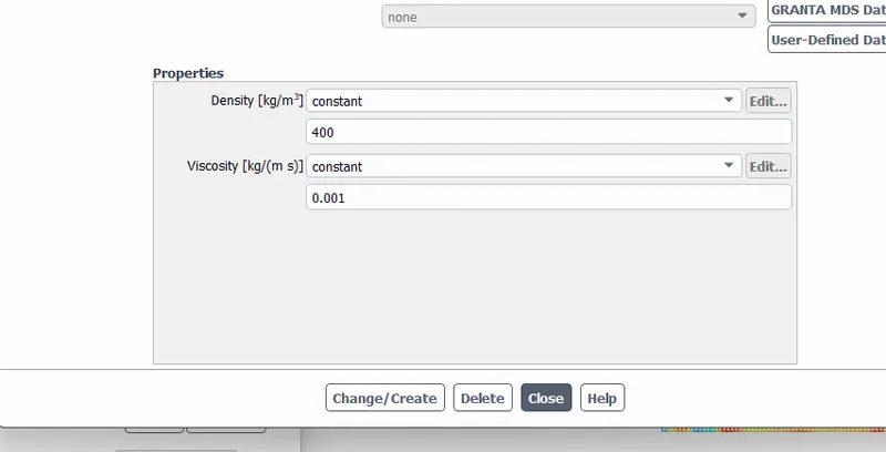
3. Run one more simulation with water and user-defined material(density = 400 kg/m³, viscosity = 0.001 kg/m-s) for refined mesh.
4. Define the Atwood Number. Find out the Atwood number for both the cases and explain how the variation in Atwood number in the above two cases affects the behavior of the instability.

Solution -

some practical CFD models that have been based on the mathematical analysis of Rayleigh Taylor waves

Kelvin–Helmholtz instability:

The theory predicts the onset of instability and transition to turbulent flow in fluids of different densities moving at various speeds. This instability occurs where there is a velocity shear or velocity difference between the interface of the two fluids.

Richtmyer–Meshkov instability:

This type of instability occurs when there is an impulsive accelaration between two fluids. This type of instability can occur when there is a shock at greater speeds. The development of the instability begins with small amplitude perturbations which initially grow linearly with time. This is followed by a nonlinear regime with bubbles appearing in the case of a light fluid penetrating a heavy fluid, and with spikes appearing in the case of a heavy fluid penetrating a light fluid. A chaotic regime eventually is reached and the two fluids mix. This instability can be considered the impulsive-acceleration limit of the Ryleigh- taylor instability.

Plateau–Rayleigh instability:

The Plateau–Rayleigh instability, often just called the Rayleigh instability, explains why and how a falling stream of fluid breaks up into smaller packets with the same volume but less surface area. It is related to the Ryleigh- taylor instability. and is part of a greater branch of fluid dynamics concerned with fluid thread breakup. This fluid instability is exploited in the design of a particular type of ink jet technology. whereby a jet of liquid is perturbed into a steady stream of droplets.The driving force of the Plateau–Rayleigh instability is that liquids, by virtue of their surface tensions, tend to minimize their surface area. A considerable amount of work has been done recently on the final pinching profile by attacking it with self- similar solutions.

Rayleigh- taylor instability simulation:

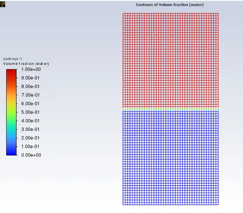
The rayleigh taylor instability occurs when the interface of two fluids with different densities when the lighter fluid is pushing the heavier fluid. In this simulation there are 2 surfaces Place over each other. The geometry for the simulation is given below:

The upper sqaure of the geometry represents water and lower square represents air. The simulation is done for transient case. At t= 0 the water in the above sqaure is resting and the air in the lower square is also resting. As the simulation is carried out the water due to gravitational effects comes down and air moves up. During this process there will be some instabilty that will occur at the surface. This simulation is performed to study the instabilities that occur at the interface.

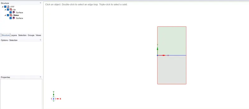
Use share topology to share the edge.

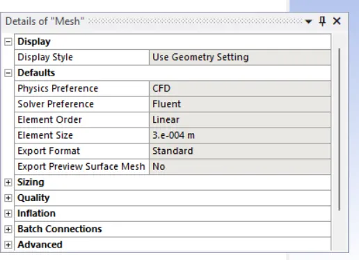
2. The Rayleigh Taylor instability simulation for 2 different mesh sizes with the base mesh being 0.5 mm

Case -1

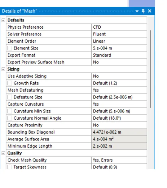
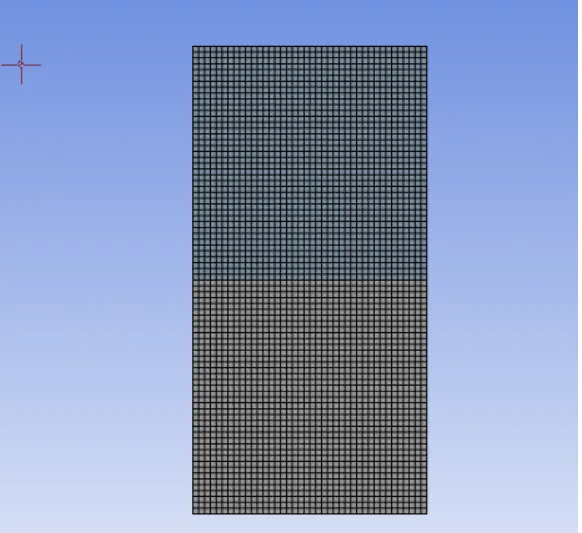
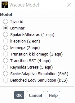
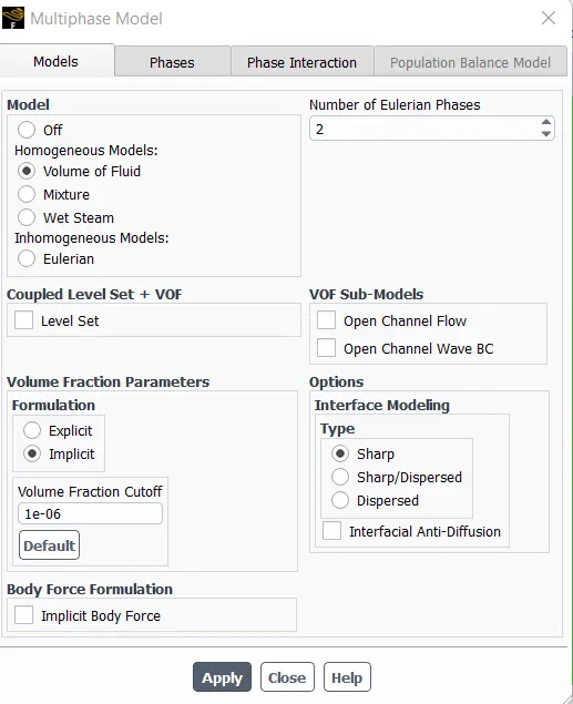
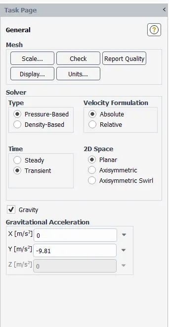
Steady approach is not suitable because it give the result after reaching the steady state.

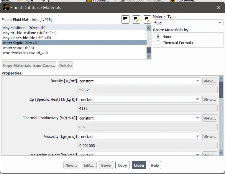
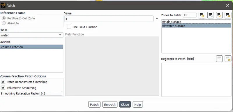
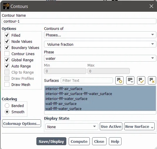
After initializing and patching the contour is created

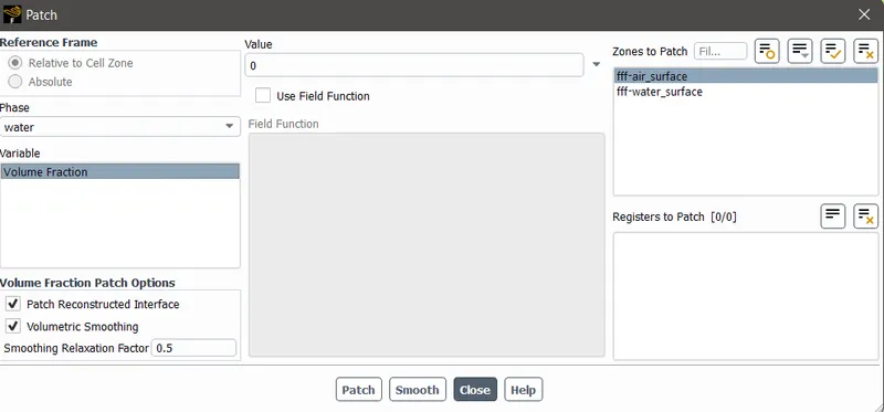
RESULT

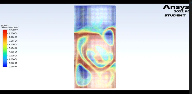
Animation link

https://drive.google.com/file/d/1PWARPd3VVKVJbRm6ZfV2jn9SAIcF_VuU/view?usp=sharing

CASE -2

Element size=0.3 mm

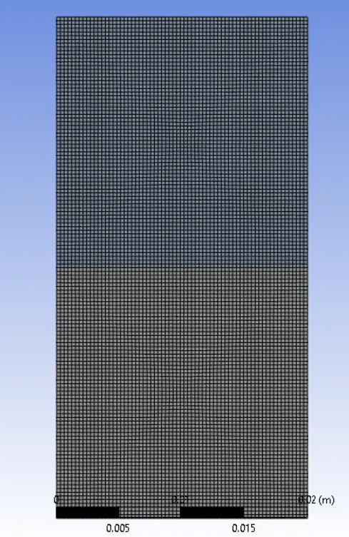
Result -

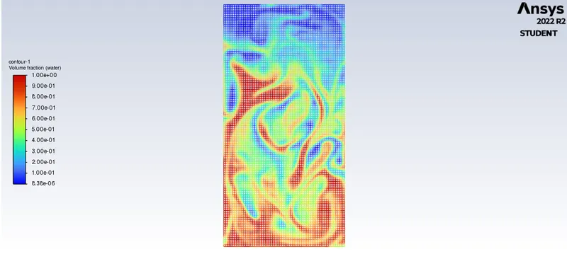
Animation link

https://drive.google.com/file/d/1nBRPZLLDI5YOyy5D9QCzu9HIgFWycanp/view?usp=sharing

3. simulation with water and user-defined material(density = 400 kg/m³, viscosity = 0.001 kg/m-s) for refined mesh.

element mesh size =0.3 mm

Steps same as above withe same finer mesh

Result

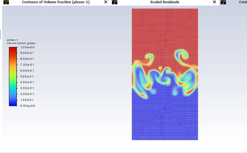
Animation link

https://drive.google.com/file/d/1WBPA-d5vH1_QE-FkSSy4O9WeV-p3hucr/view?usp=sharing

4. The Atwood number is a dimensionless number in fluid dynamics used in the study of hydrodynamic instabilities in density stratified flows. It is a dimensionless density ratio defined as..

A= (rho1-rho2)/(rho1+rho2)

where, rho1 = desnity of heavier fluid

rho2= density of lighter fluid

Application- Atwood number is an important parameter in the study of rayleigh-tayor instability and richmyer-mechkow instability. In RTI, the penetration distance of heavy fluid bubbles into the light fluid is a function of acceleration time scale, where g is the gravitational acceleration & t is the time.

So using the above formula we get Atwood NUmber as

Case 1 and Case 2 = 0.99754

Case 3 = 0.4285

Conclusion -

• As mesh become finer, the mixing becomes much clear & visible.
• The computation time also increases with increases in finer of mesh.
• Higher the atwood Number the Instabilites are sudden and Reach steady state more rapidly
• Lower the Atwood Number Instabilites Take time and Reach steady state slowly