Project 2 - Rankine cycle Simulator
Aim-
- Create a Rankine Cycle Simulator using OCTAVE/MATLAB.
- plot the corresponding T-s and h-s plots for the given set of inputs.
Theory -
The Rankine Cycle is a cycle commonly that is used to convert the pressure energy of steam into mechanical energy by using steam turbines.
Cycle’s major components
- Steam turbine
- Pump
- Stationary condenser
- Boiler
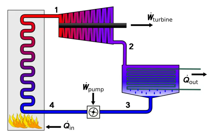
There are four processes in a Rankine cycle.
1. 1-2 Isentropic Expansion. The vapor is expanded in the turbine, thus producing work that may be converted to electricity. the expansion is limited by the temperature of the cooling medium and by the erosion of the turbine blades by liquid entrainment in the vapor stream as the process moves further into the two-phase region
2. 2-3 Isobaric Heat Rejection. The vapor-liquid mixture leaving the turbine is condensed at low pressure.
3. 3-4 Isentropic Compression. The pressure of the condensate is raised in the feed pump.
4. 4-1 Isobaric Heat Transfer. High-pressure liquid enters the boiler from the pump and is heated to the saturation temperature. Further addition of energy causes evaporation of the liquid until it is fully converted to saturated steam .
Matlab Code of rankine cycle simulator
clear all
close all
clc
%display
fprintf('        rankine cycle simulator\n')
fprintf('1-2 is an isentropic expansion\n')
fprintf('2-3 is constant pressure by heat rejection by condensor\n')
fprintf('3-4 is isentropic compression in the pump\n')
fprintf('4-1 is constant pressure heat addition in the boiler\n')
%state1
p1=input('Enter the value of pressure at turbine inlet in bar,p1= ');
T1=input('Enter the value of temperatureat turbine inlet in celcius,t1= ');
p2=input('Enter the value of pressure at condensor in bar,p2= ');
h1=XSteam('h_pT',p1,T1);
s1=XSteam('s_pT',p1,T1);
%state2
s2=s1;
sf2=XSteam('sL_P',p2);
sg2=XSteam('sv_P',p2);
x2=(s2-sf2)/(sg2-sf2);
hf2=XSteam('hL_P',p2);
hg2=XSteam('hv_P',p2);
h2=hf2+(x2*(hg2-hf2));
%state3
p3=p2;
s3=XSteam('sL_P',p3);
h3=XSteam('hL_P',p3);
%state4
s4=s3;
p4=p1;
%work done by turbine
wt=h1-h2;
%work done to run the pump
v3=XSteam('vL_P',p3);
wp=v3*(p4-p3)*100;
h4=h3+wp;
%network
w_net=wt-wp;
%heat in the system
Q_input=h1-h4;
%output heat
Q_output=h2-h3;
%thermal efficiency
Thermal_eff=(w_net/Q_input)*100;
%specific heat consumption
%SSC mass flow rate/power
SSC=(3600/w_net);
%Back Work ratio
BW=(wp/wt);
%Calculation of Temperatures at the state points
T3 = XSteam('Tsat_p', p3);
T2=T3;
cp4 = XSteam('Cp_ps', p4, s4);
cv4 = XSteam('Cv_ps', p4, s4);
k = cp4/cv4;
T4=T3/((p3/p4)^((k-1)/k));
%calculating Temperature, Entropy and Enthalpy at the vapour and liquid line
T6= XSteam('Tsat_p', p1);
s5=XSteam('sL_p', p1);
s6= XSteam('sV_p', p1);

h5=XSteam('hL_p', p1);
h6=XSteam('hv_p', p1);
T5 = T6;

%Plotting the saturation curve

T=linspace(1,T1,1000);

for i=1:length(T)

sf(i)=XSteam('sL_T', T(i));
sg(i)=XSteam('sV_T', T(i));
hf(i)=XSteam('hL_T', T(i));
hg(i)=XSteam('hV_T', T(i));
end

%plotting
figure(1)
hold on
plot([sf sg],[T T],'linewidth',1,'color','b')
plot([s1 s2 s3 s4 s5 s6 s1],[T1 T2 T3 T4 T5 T6 T1],'linewidth',1,'color','r')
text(s1,T1,'1')
text(s2,T2,'2')
text(s3,T3,'3')
text(s4,T4,'4')
text(s5,T5,'5')
text(s6,T6,'6')
xlabel('entropy')
ylabel('Temperature')
title('rankine cycle Entropy v/s temperature')
figure(2)
hold on
plot([sf sg],[hf hg],'linewidth',1,'color','b')
plot([s1 s2 s3 s4 s5 s6 s1],[h1 h2 h3 h4 h5 h6 h1],'linewidth',1,'color','r')
text(s1,h1,'1')
text(s2,h2,'2')
text(s3,h3,'3')
text(s4,h4,'4')
text(s5,h5,'5')
text(s6,h6,'6')
xlabel('entropy')
ylabel('enthalpy')
title('rankine cycle Entropy v/s temperature')
%displaying results
disp('Results');
disp('At state point 1')
fprintf('P1 is %.3f bar\n',p1)
fprintf('T1 is %.3f C\n',T1)
fprintf('h1 is %.3f kJ/kg\n',h1)
fprintf('s1 is %.3f k3/kgk\n', s1)
fprintf('\n')
disp('At state point 2')
fprintf('P2 is %.3f bar\n',p2)
fprintf('T2 is %.3f C\n', T2)
fprintf('h2 is %.3f k3/kg\n',h2)
fprintf('s2 is %.3f kJ/kgk\n', s2)
fprintf('\n')
disp('At state point 3')
fprintf('P3 is %.3f bar\n', p3)
fprintf('T3 is %.3f C\n', T3)
fprintf('h3 is %.3f kJ/kg\n',h3)
fprintf('s3 is %.3f k/kgk\n',s3)
fprintf('\n')
disp('At state point 4')
fprintf('P4 is %.3f bar\n',p4)
fprintf('T4 is %.3f c\n',T4)
fprintf('h4 is %.3f k3/kg\n',h4)
fprintf('s4 is %.3f kJ/kgk\n',s4)
fprintf('\n')
fprintf('Wt is %.3f k3/kg\n',wt)
fprintf('wp is %.3f kJ/kg\n',wp)
fprintf('Wnet is %.3f k3/kg\n',w_net)
fprintf('Thermal efficiency is %.2f Percent\n', Thermal_eff)
fprintf('ssc is %.2f kg/kWh\n',SSC)
fprintf('Back work ratio is %.3f',BW)
Output Plots and Screen
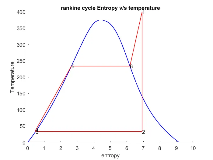
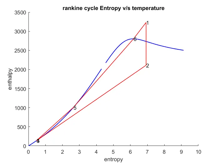
Command Window
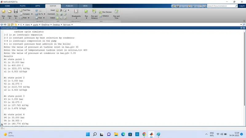
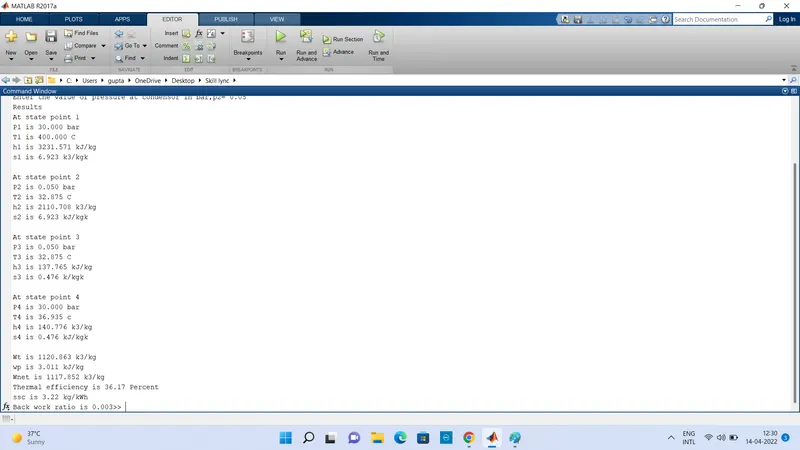
w_net =
1117.852 kJ/kg
Back work ratio =
0.003