Week 4.1 - Genetic Algorithm
A genetic algorithm (GA) is a method for solving both constrained and unconstrained optimization problems. by using the ga function we can find the minima and maxima of the function.
Syntax of ga
x = ga(function,nvars)
x = ga(function,nvars,A,b)
x = ga(function,nvars,A,b,Aeq,beq)
x = ga(function,nvars,A,b,Aeq,beq,lb,ub)
x = ga(function,nvars,A,b,Aeq,beq,lb,ub,nonlcon)
x = ga(function,nvars,A,b,Aeq,beq,lb,ub,nonlcon,options)
x = ga(function,nvars,A,b,[],[],lb,ub,nonlcon,IntCon)
x = ga(function,nvars,A,b,[],[],lb,ub,nonlcon,IntCon,options)
x = ga(problem)
[x,fval] = ga(function,nvars,...)
[x,fval,exitflag] = ga(function,nvars,...)
[x,fval,exitflag,output] = ga(function,nvars,...)
[x,fval,exitflag,output,population] = ga(function,nvars,...)
[x,fval,exitflag,output,population,scores] = ga(function,nvars,...)
x = ga(function,nvars) finds a local unconstrained minimum, x, to the objective function, function. nvars is the dimension (number of design variables) of function.
x = ga(function,nvars,A,b) finds a local minimum x to function, subject to the linear inequalities A*x ≤ b. ga evaluates the matrix product A*x as if x is transposed (A*x').
x = ga(function,nvars,A,b,Aeq,beq) finds a local minimum x to function, subject to the linear equalities Aeq*x = beq as well as A*x ≤ b. (Set A=[] and b=[] if no linear inequalities exist.) ga evaluates the matrix product Aeq*x as if x is transposed (Aeq*x').
x = ga(function,nvars,A,b,Aeq,beq,lb,ub) defines a set of lower and upper bounds on the design variables, x, so that a solution is found in the range lb ≤ x ≤ ub. (Set Aeq=[] and beq=[] if no linear equalities exist.)
x = ga(function,nvars,A,b,Aeq,beq,lb,ub,nonlcon) subjects the minimization to the constraints defined in nonlcon. The function nonlcon accepts x and returns vectors C and Ceq, representing the nonlinear inequalities and equalities respectively. ga minimizes the function such that C(x) ≤ 0 and Ceq(x) = 0. (Set lb=[] and ub=[] if no bounds exist.)
x = ga(function,nvars,A,b,Aeq,beq,lb,ub,nonlcon,options) minimizes with the default optimization parameters replaced by values in options. (Set nonlcon=[] if no nonlinear constraints exist.) Create options using optimoptions (recommended) or gaoptimset.
x = ga(function,nvars,A,b,[],[],lb,ub,nonlcon,IntCon) requires that the variables listed in IntCon take integer values.
Note: When there are integer constraints, ga does not accept linear or nonlinear equality constraints, only inequality constraints.
x = ga(function,nvars,A,b,[],[],lb,ub,nonlcon,IntCon,options) minimizes with integer constraints and with the default optimization parameters replaced by values in the options structure.
x = ga(problem) finds the minimum for problem, where problem is a structure.
[x,fval] = ga(function,nvars,...) returns fval, the value of the fitness function at x.
[x,fval,exitflag] = ga(function,nvars,...) returns exitflag, an integer identifying the reason the algorithm terminated.
MATLAB code to optimize the stalagmite function and find the global maxima of the function.
clear all
close all
clc

x=linspace(0,0.6,150);
y=linspace(0,0.6,150);
%creating 2D Array
[xx yy]=meshgrid(x,y);
for i=1:length(xx)
    for j=1:length (yy)
        input_vector(1)=xx(i,j);
        input_vector(2)=yy(i,j);
        f(i,j)=stalagmite(input_vector); %calling of fuction
    end
end
tic  %count of time
%study 1 satistical behaviour
num_cases=50;

for i=1:num_cases
    [inputs1, fop(i)]=ga(@stalagmite,2)
    xop(i)=inputs1(1);
    yop(i)=inputs1(2);
end
study1_time=toc
    figure(1)
    subplot(2,1,1)
    hold on
    surfc(x,y,f) %creating 3D surface plot
    shading interp  %smoothen the plot
    plot3(xop,yop,fop,'marker','o','markersize',3,'markerfacecolor','r')
    title('unbounded inputs')
    subplot(2,1,2)
    plot(fop)
    xlabel('iteration')
    ylabel('function minimum and maximum')

%study 2 with bounded input
num_cases=50;

for i=1:num_cases
    [inputs1, fop(i)]=ga(@stalagmite,2,[],[],[],[],[0;0],[1;1])
    xop(i)=inputs1(1);
    yop(i)=inputs1(2);
end
study2_time=toc
    figure(2)
    subplot(2,1,1)
    hold on
    surfc(x,y,f)
    shading interp
    plot3(xop,yop,fop,'marker','o','markersize',3,'markerfacecolor','r')
    title('bounded inputs')
    subplot(2,1,2)
    plot(fop)
   xlabel('iteration')
    ylabel('function minimum and maximum')
%study3 increasing iteration size
num_cases=50;
%creating optimizing options
options=optimoptions('ga');
options=optimoptions(options,'populationsize',200);

for i=1:num_cases
    [inputs1, fop(i)]=ga(@stalagmite,2,[],[],[],[],[0;0],[1;1],[],[],options)
    xop(i)=inputs1(1);
    yop(i)=inputs1(2);
end
study3_time=toc
    figure(3)
    subplot(2,1,1)
    hold on
    surfc(x,y,f)
    shading interp
    plot3(xop,yop,fop,'marker','o','markersize',3,'markerfacecolor','r')
    title('bounded inputs with more populationsize')
    subplot(2,1,2)
    plot(fop)
    xlabel('iteration')
    ylabel('function minimum and maximum')
Stalagmite function
function result=stalagmite(input_vector)
x=input_vector(1);
y=input_vector(2);
t1=(sin(5.1*pi*x+0.5)).^6;
t2=(sin(5.1*pi*y+0.5)).^6;
t3=exp((-4*log(2)*(x-0.0667).^2)/0.64);
t4=exp((-4*log(2)*(y-0.0667).^2)/0.64);
f=(t1*t2*t3*t4);
%to find maxima of function
[result]=1/(1+f);
end
Explanation of program
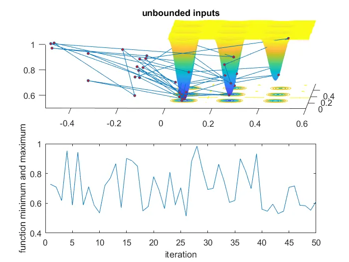
Case study 1- in this study we will run the genetic algorithm function 50 times, and will plot the output for each case by using for loop
The problem here is that the algorithm does not know the boundary condition
it will perform the algorithm for any random values.
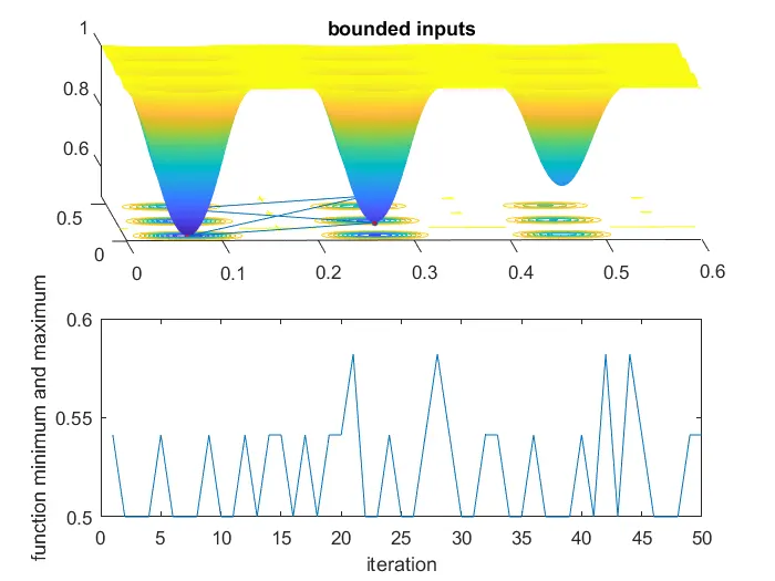
case study 2-
x = ga(function,nvars,A,b,Aeq,beq,lb,ub)
here we put lower and upper boundary values.
which gives us better results compare to study 1
case study 3-
ere we will increase the size of the population so as to get the maximum value of the function and toy reduce the fluctuation of the optimum function in the previous graph
output plots
for study 1
for study 2
for study 3
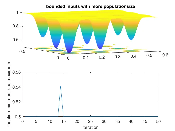
from study 3 we get
global maxima = 0.5414
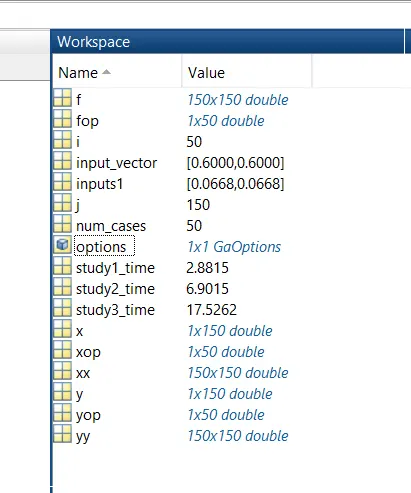
study1 time = 2.8815 sec
study2 time = 6.9015 sec
study3 time = 17.5262 sec