Week 5 - Rayleigh Taylor Instability

Numerical Analysis of Rayleigh Taylor Instability

AIM

1. Perform the Rayleigh Taylor instability simulation for 2 different mesh sizes with the base mesh being 0.5 mm. Choose Air and Water for this simulation.
2. Perform another simulation with water and user-defined material(density = 400 kg/m³, viscosity = 0.001 kg/m-s) for refined mesh.
3. Find out the Atwood number for the above cases and explain how the variation in the Atwood number in the above two cases affects the behavior of the instability.

THEORY

Rayleigh–Taylor Instability :

Rayleigh–Taylor Instability (RTI) occurs at an interface between two fluids of different densities when the lighter fluid is pushing through the heavier fluid. It is a dynamic process where 2 fluids seek to reduce their combined potential energy.

Water suspended above oil, mushroom clouds from nuclear explosions and volcanic eruptions, instabilities in plasma fusion reactors, and inertial confinement fusion are a few examples of RTI.

Kelvin–Helmholtz Instability :

Kelvin–Helmholtz Instability is another instability that is related to Rayleigh Taylor waves. This occurs when there is a velocity difference or velocity shear in a continuous fluid. This instability is observed in the cloud formations and Red spot on Jupiter.

Richtmyer–Meshkov Instability :

Richtmyer–Meshkov instability (RMI) occurs when 2 fluids having different densities are accelerated by a shockwave or any other impulsive methods. This instability can be considered as an impulsive acceleration limit of RTI. Examples of this instability include Magnetized target fusion, Inertial confinement fusion, and supersonic combustion in a Scramjet.

Some CFD models used to study these instabilities involving 2 fluids are,

1. Buoyancy Drag model
2. BHR Model
3. K-l model

Atwood Number :

The Atwood number (A) is a dimensionless number that gives us an idea about the density difference between 2 fluids and is used in the study of hydrodynamic instabilities. It is a density ratio and can be written as

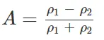ρ1= density of the heavier fluid and ρ2= density of the lighter fluid

Atwood number is a significant parameter in the study of Rayleigh–Taylor instability and Richtmyer–Meshkov instability. It gives information regarding the penetration of heavier fluid bubbles into the lighter fluid bubbles in RTI through the acceleration time scale function.

MODELLING APPROACH

• Water and air are taken as fluids for case 1 and case 2. For case 1, the base mesh size is 0.5mm and for case 2 mesh size is 0.1mm.
• We are using the Transient solver in place of the Steady-state solver for this analysis as we are more interested in the intermediate stages and not just the end result.
• Under the Multiphase tab, we select the Volume of fluid method to run simulations.
• The implicit method is chosen. Air is selected as the primary phase and water is selected as the secondary phase.
• After hybrid initialization is completed, we need to patch the geometry to observe the volume fraction of water throughout the simulation.
• Simulations are performed with the SIMPLE algorithm using the 2nd-order Upwind scheme.

PRE-PROCESSING

Geometry

• Open Spaceclaim
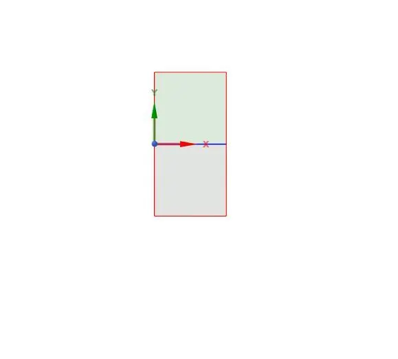
• Using the Rectangle option from the Design tab, create a rectangle from the origin.
• Then use the Pull tool to convert the rectangle to a 3D surface.
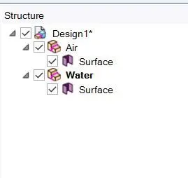
• Now create a new component and again create a rectangle on top of the first one.
• Use the Share tool to share the interface between both surfaces.

Mesh :

• Open the Mesh section
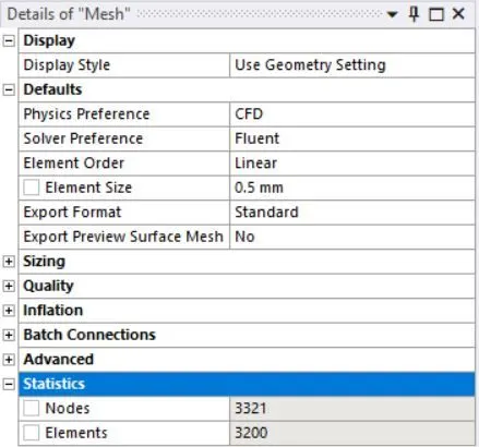
• Edit the mesh element size according to the case requirement.

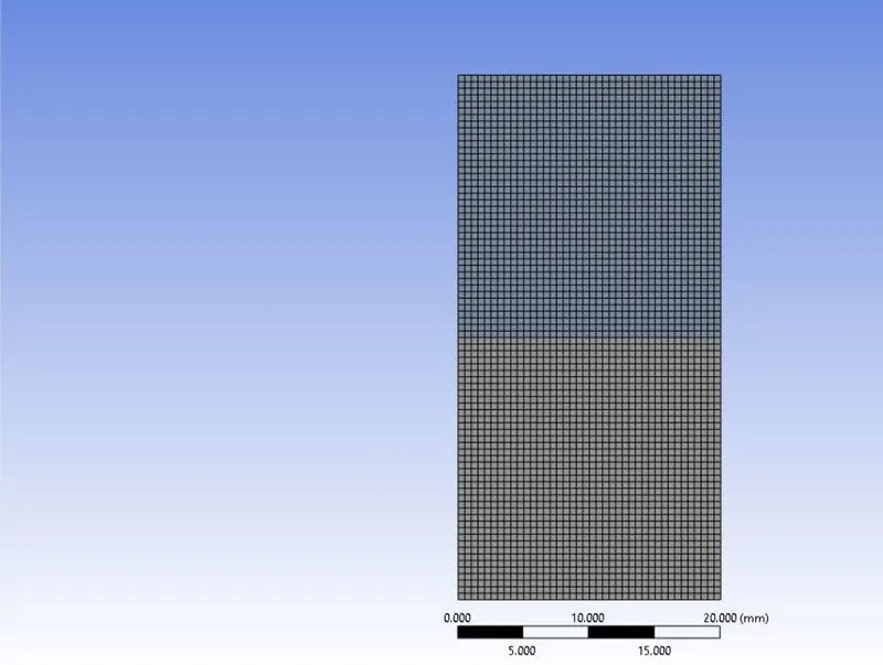
Setup

1.	Solver type	Pressure based
2.	Solver time	Transient
3.	Multiphase	ON (Volume of Fluid)
4.	Viscous model	Laminar
5.	Material	Air & Water
6.	Primary phase	Air
7.	Secondary phase	Water
8.	Energy	OFF
9.	Method	Coupled
10.	Patching	Done

• Gravity is set as -9.81 m/s2
• Add contour for volume fraction.
• Add solution animation and run the simulation after setting the correct timestep.
• Check the Autosave option so that the animation can be retrieved from CFD Post.

RESULTS

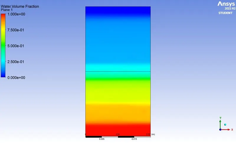
Case 1

1. Mesh element size - 0.5mm
2. Number of elements - 3200
3. Time step size - 0.01
4. Number of time steps - 500

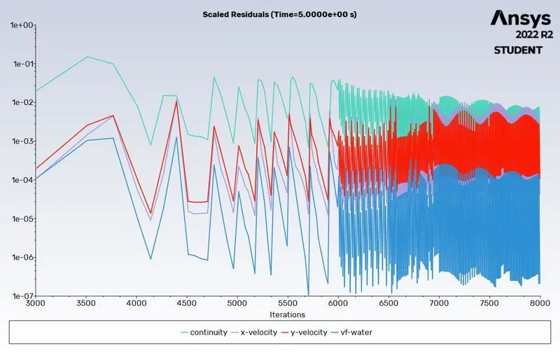
• Residuals

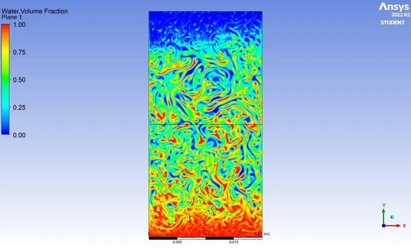
• Volume Fraction at different number of time steps

At 20

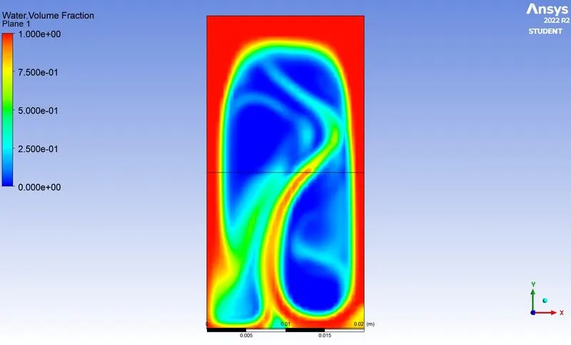
At 100

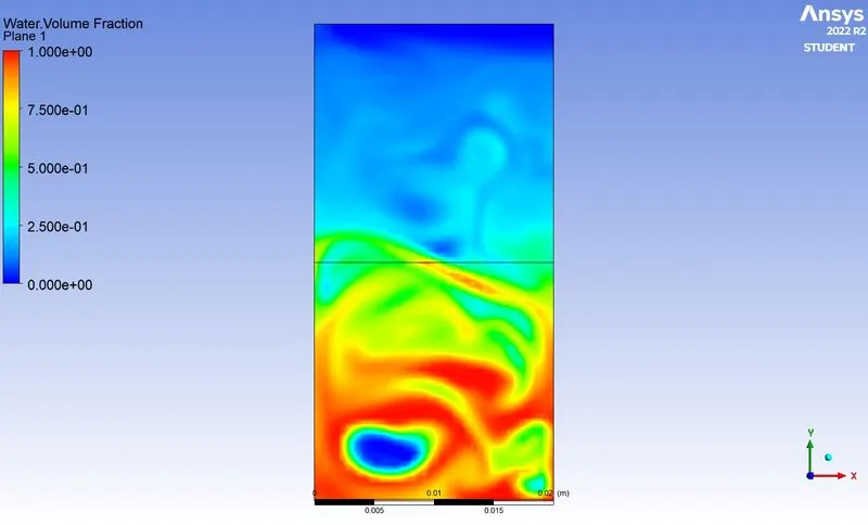
At 500

Case 2

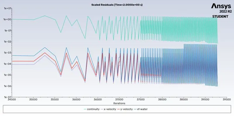
1. Mesh element size - 0.1mm
2. Number of elements - 8000
3. Time step size - 0.001
4. Number of time steps - 2000

• Residuals

• Volume Fraction at different number of time steps

At 100

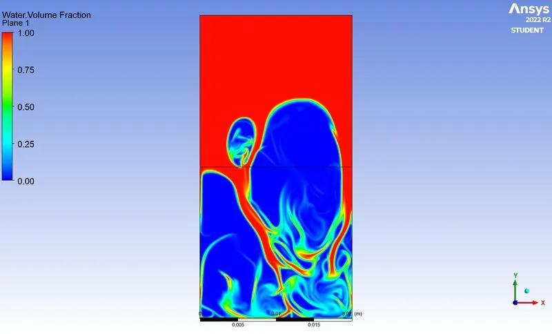
At 200

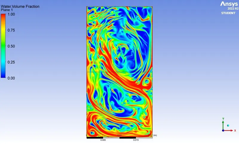
At 2000

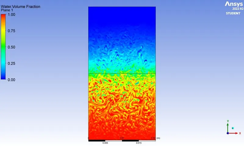
Case 3

1. Mesh element size - 0.1mm
2. Number of elements - 8000
3. Time step size - 0.001
4. Number of time steps - 2000
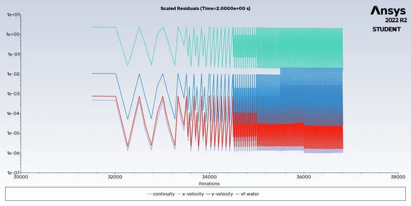
5. Primary phase - user-defined fluid (400kg/m3)

• Residuals

• Volume Fraction at different number of time steps

At 200

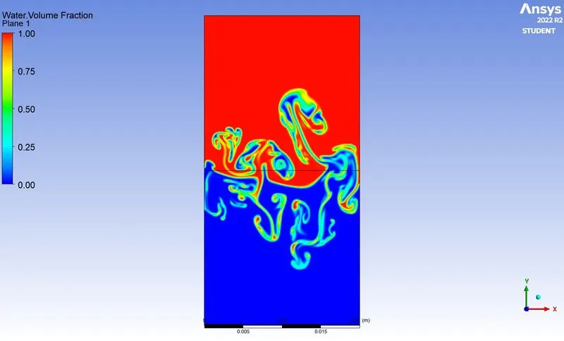
At 500

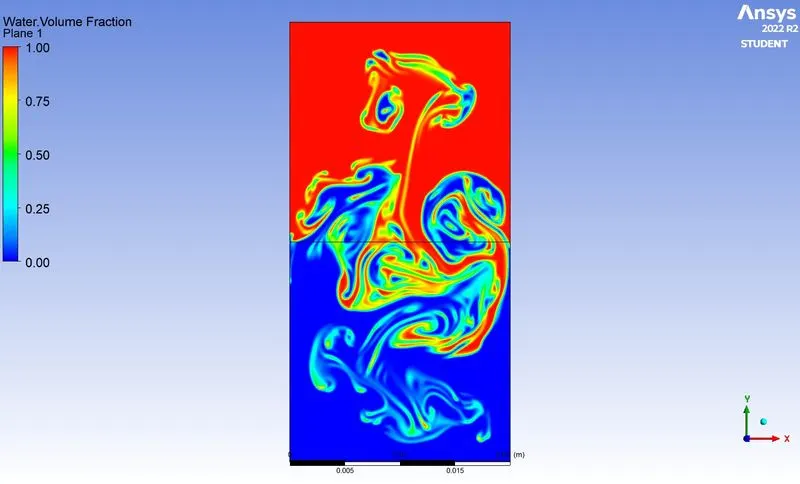
At 2000

Atwood number

• Density of water is 998 8.2 Kg/m³
• Density of air is 1.225 Kg/m³
• Density of custom fluid is 400 Kg/m³

For Case 1 and Case 2,

Atwood number =`(998.2-1.225)/(998.2+1.225)`= 0.9975

For Case 3,

Atwood number = `(998.2-400)/(998.2+400)` = 0.427

Animation videos (Google drive links)

1. Case 1 - https://drive.google.com/file/d/1mlmOiKPvhAfT8eMDZ5kKGD9_ulUIHZmi/view?usp=sharing
2. Case 2 - https://drive.google.com/file/d/1pHv7gXMqbb9kIUt3wU-riAucbDoBKsZu/view?usp=sharing
3. Case 3 - https://drive.google.com/file/d/15AqjTp7PHyjwjJNYek6EOgFngz3kSUL3/view?usp=sharing

CONCLUSIONS

1. Finer mesh gives better results than coarser mesh and we can observe it in cases 1 and 2. But the computational time taken for the fluid to settle down is more in the case of finer mesh.
2. The transient approach is preferred over the steady-state approach as we needed to study how the mixing was taking place in intermediate stages.
3. The Atwood number for cases 1 and 2 is closer to 1(0.9975 ). Atwood number closer to one would have a higher density difference creating bubbles and plumes. This is evident from the animation video and timestep images.
4. The Atwood number for case 3 is closer to 0 (0.427). In this scenario, the density difference is low and we can see symmetrical mixing with the shape of a finger.
5. For the same number of time steps (2000), we can observe that in case 3 it takes more time for the fluid to settle because of the higher density of the user-defined fluid.
6. A low timestep value will result in the floating point exception error.

REFERENCES

1. Indrashis Saha 2020 study of Rayleigh Taylor Instability with the help of CFD simulation.
2. D.L. Youngs, Numerical simulation of turbulent mixing by Rayleigh–Taylor instability, Physica D 12 (1984) 32–44.
3. Budiana, E. P. (2020) Meshless numerical model based on radial basis function (RBF) method to simulate the Rayleigh–Taylor instability (RTI). Computers & Fluids, 201, 104472.
4. D. Sharp, An overview of Rayleigh–Taylor instability, Physica D 12 (1984) 3–18.
5. Hirt, C. W., & Nichols, B. D. (1981) Volume of fluid (VOF) method for the dynamics of free boundaries. Journal of computational physics, 39(1), 201