Week 5 - Rayleigh Taylor Instability

OBJECTIVE:

The objective of this project is to perform Rayleigh Taylor Instability simulation.

Theory:

Rayleigh Taylor Instability:

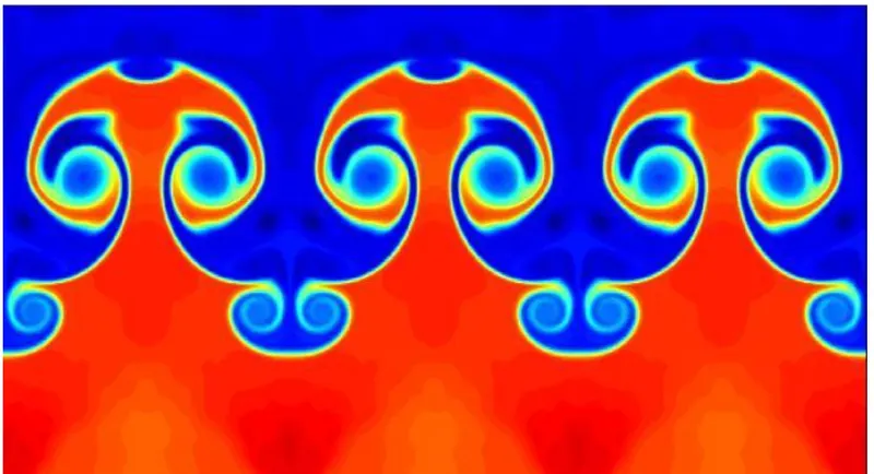
Rayleigh Taylor Instability (RTI) is a phenomenon that occurs at the interface of fluids of different densities wherein the lighter fluid pushes the heavier fluid due to the density difference. It is a dynamic process wherein the system tries to reduce its combined potential energy. Initially, the system is in a state of hydrostatic equilibrium, in which the heavier fluid (ex: water) sits atop a lighter fluid (ex: air) in a constant gravitational field. As the RTI develops, the initial perturbations progress from a linear growth phase, eventually developing "plumes" flowing upwards (in the gravitational buoyancy sense) and "spikes" falling downwards. In the linear phase, equations can be linearized and the amplitude of perturbations is growing exponentially with time. In the non-linear phase, the perturbation amplitude is too large for the non-linear terms to be neglected. In general, the density disparity between the fluids determines the structure of the subsequent non-linear RT instability flows (assuming other variables such as surface tension and viscosity are negligible here). Examples include supernova, water suspended atop oil, mushroom clouds formed due to volcanic eruptions.

Some of the practical CFD models that have been based on mathematical analysis of RT waves...

1. Kelvin-Helmholtz instability.
2. Richtmyer-Meshkov instability.
3. Plateau-Rayleigh instability.

Kelvin-Helmholtz instability:

This instability typically occurs when there is velocity shear in a single continuous fluid, or additionally where there is a velocity difference across the interface between two fluids. A common example is seen when wind blows across a water surface; the instability constant is able to manifest itself through waves on water surface. The Kelvin-Helmholtz instability is not only restricted to a water surface as clouds, but is evident through other natural phenomena as ocean and the sun's corona.

Richtmyer-Meshkov instability:

This occurs when two fluids of different density are impulsively accelerated. Normally this is by the passage of a shock wave. The development of the instability begins with small amplitude perturbations which initially grow linearly with time. This is followed by a nonlinear regime with bubbles appearing in the case of a light fluid penetrating a heavy fluid, and with spikes appearing in the case of a heavy fluid penetrating a light fluid. A chaotic regime eventually is reached and the two fluids mix. This instability can be considered the impulsive-acceleration limit of the Rayleigh Taylor instability.

Plateau-Rayleigh instability:

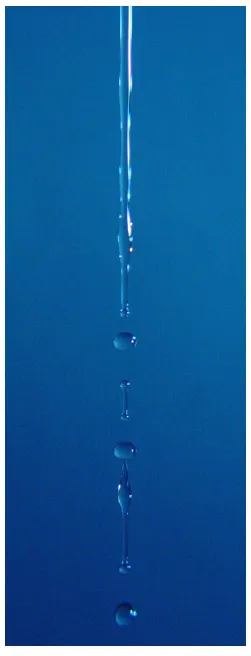
This instability, often just called the Rayleigh instability, explains why and how a falling stream of fluid breaks up into smaller packets with the same volume but less surface area. It is related to the RTI and is part of a greater branch of fluid dynamics concerned with fluid thread breakup. This fluid instability is exploited in the design of a particular type of ink jet technology whereby a jet of liquid is perturbed into a steady stream of droplets. The driving force of the Plateau–Rayleigh instability is that liquids, by virtue of their surface tension, tend to minimize their surface area.

Simulation Procedure:

1: Pre-Processing.

• Open Ansys Workbench→under Analysis system select Fluid flow(fluent) drag and drop it in Project schematic → Geometry → New spaceclaim geometry.
• First creating a rectangular sketch of 20x20 mm, which will be acting as the fluid medium.
• Then use the Pull option to make the 2d sketch into a 2d model.
• We are creating two rectangular sketches, the one at the top will act as water medium and the one at the bottom will be acting air medium.
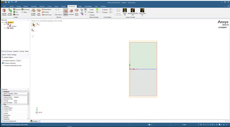
• Since we have defined a separate fluid volume, we need to share the nodes between these two bodies which will be created while meshing, to share the nodes we are using Share topology option.

Created geometry with shared topology:

2: Meshing.

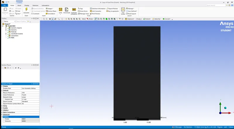
• We will proceed with mesh generation for required mesh element length using the Sizing and Inflation options. Mesh → Details of “Mesh” → Element Size then specify the required mesh length.
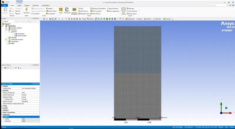
• In this case we are creating two meshes, one 0.5 mm base mesh and one with 0.1mm refined mesh.

0.5 mm Base Mesh:

0.1 mm Refined Mesh:

3: Simulation.

• Setting up for Physics. Choose pressure-based solver and Transient state condition.
• Viscous model `rarr` Laminar.
• Select the materials water & air from fluent database.
• Since the Rayleigh table simulation depends on gravity, enable gravity acting in y axis= -9.81 m/s^2
• Select volume of fluid method under multiphase option, define number of phases are 2, one is water & one is air.
• Select implicit method and rename the phases as air & water.
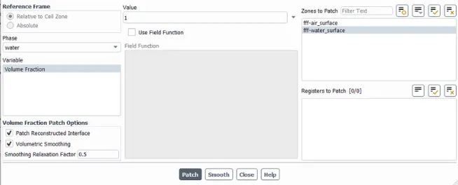
• Initialization the simulation and perform patch on water phase with volume fraction value for water as 1 and for air as 0.
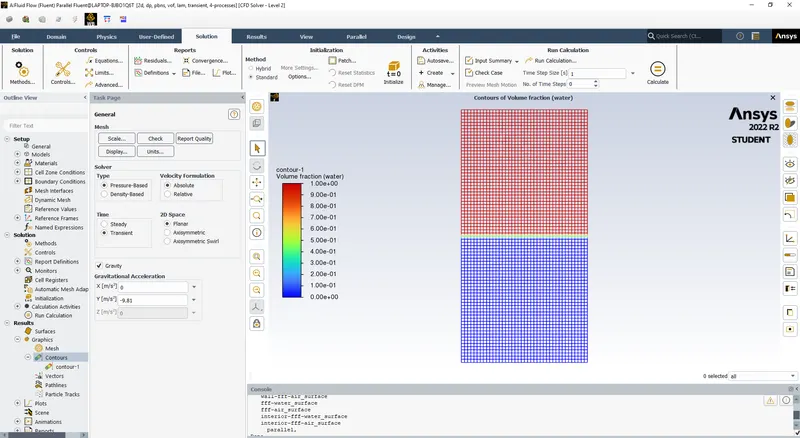
• Create a contour plot of water phase to study the RTI.

Case 1: 0.5 mm Base Mesh.

Time step size(s)=0.01.

No. Of time step=500.

Initial Contour:

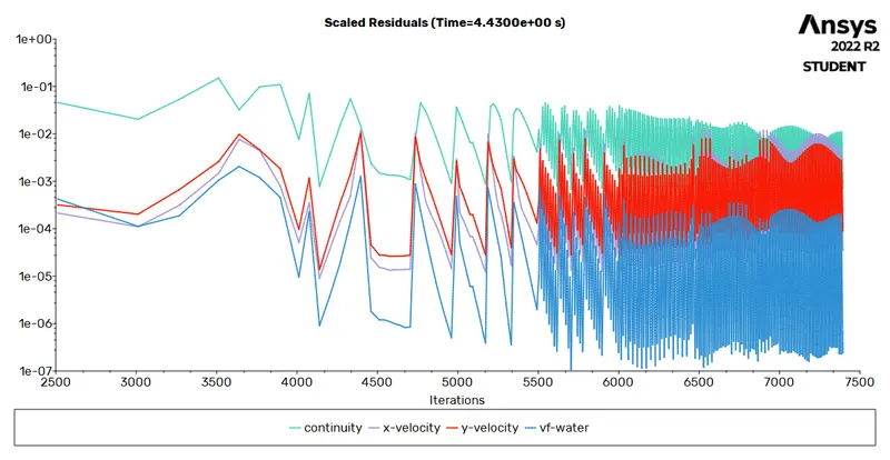
Residual Plot:

Animation:

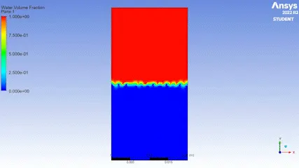
Case 2: 0.1 mm Refined Mesh.

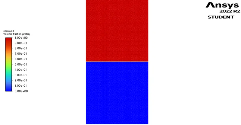
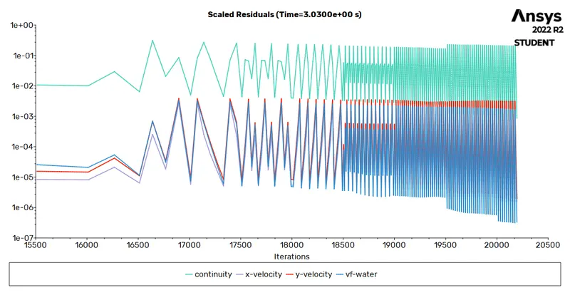
Time step size(s)=0.003.

No. Of time step=1500.

Initial Contour:

Residual Plot:

Animation:

Case 3: Use defined material.

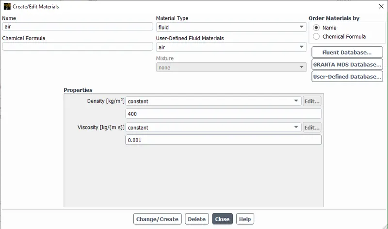
Define a new material under materials and specify the given fluid properties.

Time step size(s)=0.003.

No. Of time step=2000.

Initial Contour:

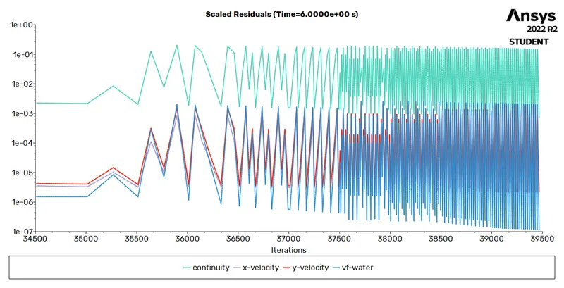
Residual Plot:

Animation:

Atwood Number:

The Atwood number is a dimensionless number in fluid dynamics used in the study of hydrodynamic instabilities in density stratified flows. It is a dimensionless density ratio defined as...

`A= (rho1-rho2)/(rho1+rho2)`

where, rho1 = density of heavier fluid

rho2= density of lighter fluid

Application- Atwood number is an important parameter in the study of Rayleigh Tayor instability in RTI, the penetration distance of heavy fluid bubbles into the light fluid is a function of acceleration time scale,

`A g t^2`

where g is the gravitational acceleration & t is the time.

For Case 1&2:

Density of heavier fluid(water)=998.2 kg/m^3. `

Density of lighter fluid(air)= 1.225 kg/m^3. `

`A=(rho1-rho2)/(rho1+rho2)=(998.2-1.225)/(998.2+1.225)=0.9975.`

For Case 3:

Density of heavier fluid(water)=998.2 kg/m^3.

User Defined Material Density=400 kg/m^3.

`A=(rho1-rho2)/(rho1+rho2) = (998.2-400)/ (998.2+400)=0.4279.`

CONCLUSION:

• From the above cases, we observe that finer mesh captures the instability better than the coarse mesh, but it takes more time for the heavier fluid to settle down. As computational time is long but produces results with better accuracy.
• Since the simulation involves capturing instabilities that are changing in an unpredictable manner as a function of time, the transient approach is preferred over the steady-state approach.
• The Atwood no validates the CFD simulation as it is observed. In the case of water and air mixing, bubble formation takes place, whereas in the other case no bubble takes place.