Week 5 - Rayleigh Taylor Instability
The aim of this exercise is to perform rayleigh taylor instability simulation for two different mesh sies and comparing the results. Also, it is required to be known as why steady state simulation method cannot be used for the purpose and running another simulation with an unser define material.
Rayleigh taylor instability is the study of mixing of two fluids where one fluid is heavier than the other and is a dynamic process where the mixing of the two fluids is studied to analyse the reduction in the combined potential energy. Rayleigh taylor instability is used in many practical cfd applications such as the inertial confinement fusion capsules (ICF), supernovae, study of turbulence models for buoyancy driven flows, mixing experiments suxh as kelvin-helmholtz instability, ritchmyer-meshkov instability where the ritchmyer-meshkov model is used to study the instability that occurs when two different fluids of different densities are accelerated impulsively (RMI). These models are adapted for cfd calculations to study the behaviour of fluids of different densities and their inter-mixing.
To perform the actual simulation, we have to create 2 surfaces on top of one another, where each represent the fluids being used. We create 20x20 surfaces where the bottom surface represents the lighter fluid which in our case is air, and the top surface is water. We use the pull tool to create surfaces, put them under a single branch, enable share topology for both and then go to meshing.
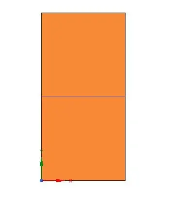
Then, we generate a baseline mesh to check the mesh quality and enter the necessary mesh parameters (sizing) according to our preference and generate the actual mesh.
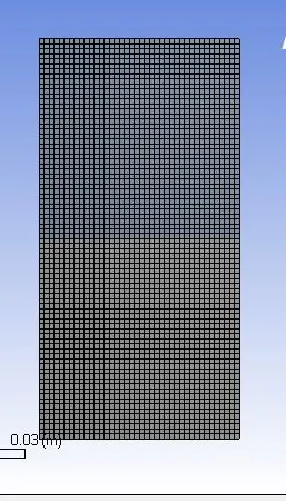
Now in setup, we check the mesh quality, then under setiing up domain, we use transcient pressure based, absolute solver and laminar viscous model. We choose gravity under operating conditions and provide the value since our gravity lies in the y direction. Under multiphase, we choose volume of fluid, implicit method and this is for 2 eulerian phases which is air and water. Under materials, we choose water and air for the first case and under phases, we choose the corresponding fluid which have been specified. Now, we initialize the simulation, specify the necessary plots we require, and animations. Then we patch and specify the values for each fluid and initialize the solution. Now, we run the simulation for fixed time stepping method, and step size of 0.005 whith number of time steps 1500.
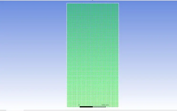
Case 1: Mesh size = 0.5mm
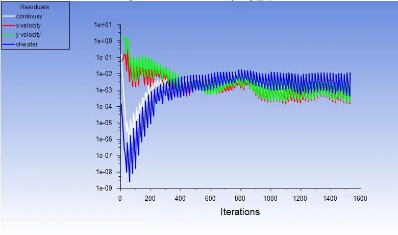
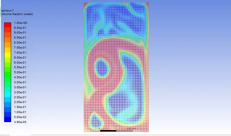
https://drive.google.com/file/d/1oTh8Kte826tin_AfvtSdROYfJaRTXQGk/view?usp=sharing
Case 2: mesh size = 0.25mm
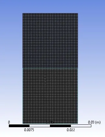
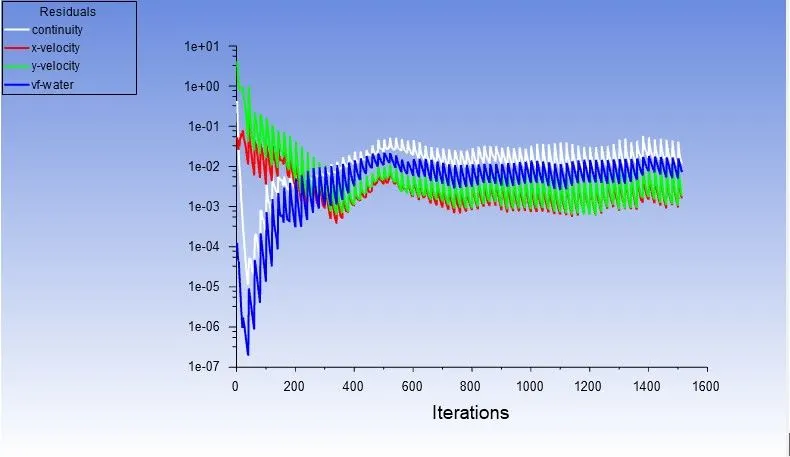
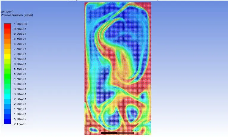
https://drive.google.com/file/d/1-GD61UdK2yUKhYxUhZB1qI2yLiEvM82Y/view?usp=sharing
Case 3: Mesh size = 0.25mm, user defined material
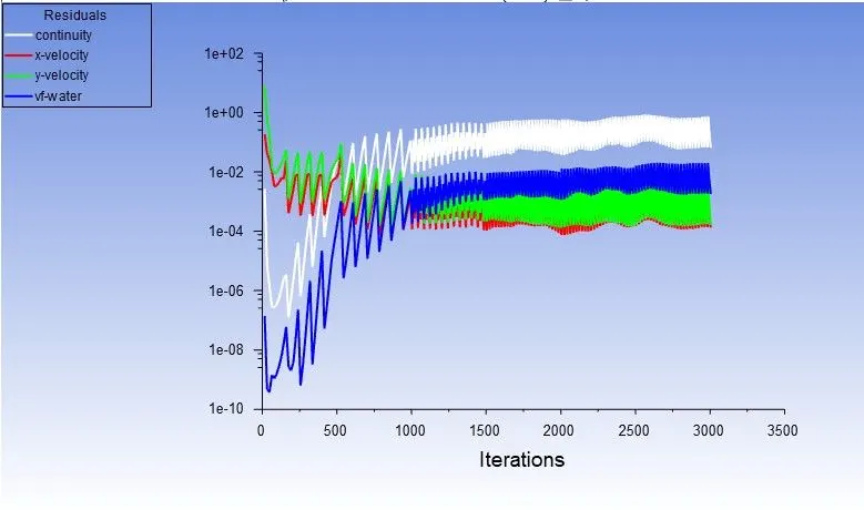
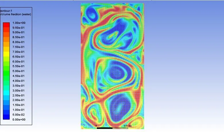
https://drive.google.com/file/d/1bQioZTw4zfVJeiT_rCwTgvOFn8oLWMDL/view?usp=sharing
In all the cases from which the results are obtained, it is evident that rayleigh taylor instability occurs at the intersection where the fluid with higher density experiences a push from the fluid with lower density, and resulting in shock waves at the area of intersection. In the first case, where the lighter fluid is air, air bubble formation takes place which surrounds the water medium and mixing is observed. When the mesh size is reduced, from 0.5mm to 0.25 mm, it is observed that the results at the interference is much more clear and simulation time is longer than the previous one. It is also observed that as the air bubbles are formed, water replaces air and in the third case the user defined material replaces water and shock wave formation is observed.
The reason for choosing transcient type instead of steady state is that whenever the results required are only regarding the final equilibrium state, then steady stae type simulation is done. But, in our case, we need to analyse the fluid trasnsition from the start to end and the development of shock waves at each given time intervals. Also, the movement of the fluids can be observed rather than only the final results, therefore prompting us to use transcient solvers.
Atwood number is a dimensionless number used to study the hydrodynamic instabilities in density based flows. It is given as :
`A = (rho_1 - rho_2)/(rho_1 + rho_2)` where `rho_1`is the density of heavier fluid and `rho_2` the density of lighter fluid.
In our 1st case: A = (1000 - 1.2754) / (1000 + 1.2754) = 0.9974
For case 3: A = (1000-400)/(1000+400) =0.4285
Atwood number for all the cases is important since we can understand the phenomenon of instability behaviour as when when atwood number tends to the value of 1, lighter fluids take form of bubbles and when it tends to 0, instability flow takes the form of symmetry.
In our cases, for case 1 and two, the the atwood number tends to 1 which is why we observe the bubbles and in third case, where atwood number tends to 0, we observe symmetry form of instability.