Week 5 - Rayleigh Taylor Instability
AIM:- The project aims to discuss Rayleigh-Taylor Instability.
OBJECTIVE:- The objectives are –
- First, We discuss some practical CFD models that have been based on the mathematical analysis of Rayleigh Taylor waves, and also we explain how these mathematical models have been adapted for CFD calculations.
- We perform the Rayleigh Taylor instability simulation for two different mesh sizes with the base mesh being 0.5 mm. We also compare those results by showing the animations. Also, We explain why a steady-state approach might not be suitable for these types of simulations. Here we choose Air and Water for the simulation.
- Here We run one more simulation with water and user-defined material(density = 400 kg/m3, viscosity = 0.001 kg/m-s) for refined mesh.
- We define the Atwood Number and also find out the Atwood number for both the cases and explain how the variation in the Atwood number in the above two cases affects the behavior of the instability.
INTRODUCTION:- In Multiphase flow, dynamic variables like velocity, viscosity, pressure, and density are generally used to explain the movement of fluids under the gravitational field. Multiphase flows take place in nuclear geothermal power plants, food processing industries, and many others. One of the basic examples is Rayleigh Taylor's Instability. The instability of a heavy fluid layer supported by a light one is generally known as Rayleigh-Taylor instability. It can occur under gravity or an acceleration of the fluid system in the direction of the denser fluid.
Because of the transient nature of the RT instabilities in common situations, its physical significance may have escaped attention for a long time. The RTI phenomenon was initially introduced by Rayleigh in 1883 and later was observed for all accelerated fluids by Taylor in 1950.
The first experiments by Lewis have shown three subsequent stages in the evaluation of an unstable air-water interface. The initial phase of exponential growth is followed, first, by a transition phase of bubble formation and then by an asymptotic stage of rising air columns. One should clearly distinguish between the instability problem, related to the initial phase, and the mixing problem, related to the asymptotic phase. In the instability problem, one is mainly concerned with the modification of instability growth rates by various physical effects. In contrast, the mixing problem is addressed by the penetration of perturbation fronts through the liquid.
Presently a large number of numerical techniques were introduced to simulate RTI including the boundary integral methods( Baker et al. 1984), the front tracking methods( Liu et al. 2007, Terashima and Tryggvason 2009), volume of fluid methods(Hirt and Nichols 1981, Gopala and BGMvan 2008, Raessi et al. 2010) and phase field methods(Ding et al. 2007, Chiu and Lin 2011, Lee et al. 2011, Kim 2005). Cheng et al. 2012 numerically simulated RTI by using a moving particle semi-implicit method that was well-validated with experimental results. The discontinuous Galerkin method was used to simulate the multi-layered Richtmyer-Meshkov and RTI problems(Henry de Frahen et al. 2015). Tryggvason 1988 used Lagrangian-Eulerian vortex methods for simulating the dynamics of perturbation in a two-fluid model. Zhang 1991 conducted a numerical investigation to study the motion of spikes in RT interfaces by applying the front tracking method on 2D Euler equations. Talat et al.2018 introduced the diffuse approximated method(DAM) and phase-field formulation for solving the 2D RTI problem where the fluids were assumed as incompressible and immiscible. Lee et al. 2011 used a phase-field method with periodic boundary conditions to simulate the dynamics of the RT interface which was based on coupled solving of both Navier Stokes equation and Cahn-Hilliard equation in the terms of all the primitive parameters or variables in the 2D staggered grid. Gou et al. 2018 used the multiphase moving particle semi-implicit(MMPS) with periodic boundary conditions to simulate RTI of the immiscible two-phase incompressible fluid. The effect of initial perturbation wavelength, surface tension, and the Atwood Number was investigated in the single-mode RTI problem and it was observed that the numerical results were in good agreement with the analytical results.
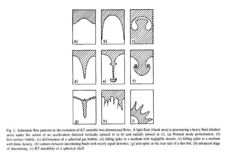
An overview of characteristic flow patterns in the evolution of RT instabilities is given by the schematic drawing in fig(1) –
However, the present study is based on the Finite Element method to simulate the interface evolution of RT Instability. Here in this study, the 2D geometry is itself constructed in Spaceclaim and a computational mesh is generated. The meshing file is imported in the fluent and a grid dependency test was performed and the results of the interfacial evolution of RTI are captured at different flow times and compared. The governing equations for the RTI were the modified form of both the Navier-Stokes equation and the Cahn-Hilliard equation. The spatial discretization involves a least-square cell-based for the gradient and for the time derivative, the first-order implicit scheme was used to solve the governing equations. A SIMPLE scheme was employed to overcome the pressure velocity coupling. In this study, the density of the secondary phase is altered with the incorporation of user-defined material resulting in variation of Atwood Number. The results of the grid dependency study and the variation of Atwood Numbers are carefully observed and reported in the present literature.
GOVERNING EQUATIONS:-
The governing equations for the RTI problem are the Navier-Stokes equations, the continuity and the Cahn-Hilliard equation which are non-dimensional form.
`(∂u)/(∂t) + u (∂u)/(∂x)+ v (∂u)/(∂y) = -1/ρ_(c) (∂p)/(∂x)+ 1/(Re*ρ_(c)) ((∂^2 u)/(∂x^2 )+(∂^2 u)/(∂y^2 ))`
`(∂v)/(∂t)+u (∂v)/(∂x)+v (∂v)/(∂y) = -1/ρ_(c) (∂p)/(∂y)+ 1/(Re*ρ_(c) ) ((∂^2 v)/(∂x^2 )+(∂^2 v)/(∂y^2 ))+ g/(Fr)`
`(∂u)/(∂x)+(∂v)/(∂y)=0`
`(∂c)/(∂t)+u (∂c)/(∂x)+v (∂c)/(∂y)= 1/(Pe) ((∂^2 μ)/(∂x^2 )+(∂^2 μ)/(∂y^2 ))`
`μ=c^3- c_h^2 ((∂^2 c)/(∂x^2 )+(∂^2 c)/(∂y^2 ))`
The above equations can be reduced into non-dimensionalized form as follows
`x^'= x/L_c ,u^'= u/U_c ,t^'= (tU_c)/L_c ,ρ^'= ρ/ρ_c ,p^'= p/(ρ_c v_c^(2 ) ) ,η^'= η/η_c ,g^'= (g/g_c) , μ^'= μ/μ_c`
Where all dot values represent non-dimensional values. The Reynolds number ( Re ), Peclet number ( Pe ), Cahn number ( `C_h` ), and Froude number ( Fr ) are defined as
`Re = (ρ_c U_c L_c)/η_c , Pe = (U_c L_c)/(Mμ) , C_h= √(ϵ/(αL_c )) , Fr= U_c/(√gL_c)`
The periodic boundary conditions are used on the left and the right boundaries ( x = 0 and x = L ), and `u=v= (∂p)/(∂y)= (∂c)/(∂y)= (∂μ)/(∂y)=0, (∂p)/(∂y)= -ρ/(Fr)`. Following this, the pressure velocity is coupled to solve the momentum equation. Here the intermediate values do not satisfy the mass continuity equation for which the intermediate velocities are corrected by pressure terms. After finishing with the calculation of u, v, and p, concentration, c, and chemical potential `mu` and Cahn-Hilliard equations are solved by a semi-implicit scheme which is followed by spatial discretization of momentum equation by second-order upwind and pressure by PRESTO.
PROJECT DESCRIPTION:-
First, we discuss some practical CFD models that have been based on the mathematical analysis of Rayleigh Taylor waves
- Kelvin-Helmholtz Instability
- Richtmyer-Meshkov Instability
- Plateau-Rayleigh Instability
Kelvin–Helmholtz instability- The Kelvin-Helmholtz Instability is a fluid instability that occurs when there is velocity shear in a single continuous fluid or a velocity difference across the interface between two fluids. Kelvin-Helmholtz instabilities are visible in the atmospheres of planets and moons, such as in cloud formations on Earth.
In situations where there is a state of static stability, evident by heavier fluids found below than the lower fluid, the Rayleigh-Taylor instability can be ignored as the Kelvin–Helmholtz instability is sufficient given the conditions. Numerically, the Kelvin–Helmholtz instability is simulated in a temporal or a spatial approach. In the temporal approach, the flow is considered in a periodic (cyclic) box "moving" at mean speed (absolute instability). In the spatial approach, simulations mimic a lab experiment with natural inlet and outlet conditions (convective instability).
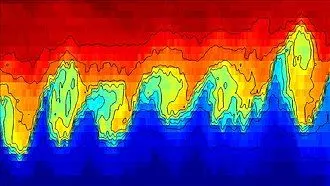

Richtmyer–Meshkov instability (RMI)- The Richtmyer-Meshkov Instability occurs when two fluids of different densities are impulsively accelerated. Normally this is by the passage of a shock wave.
The development of the instability starts with small amplitude perturbations which initially grow linearly with time. This is followed by a nonlinear regime with bubbles appearing in the case of a light fluid penetrating a heavy fluid, and spikes appearing in the case of a heavy fluid penetrating a light fluid. A chaotic regime eventually is reached and the two fluids mix. This instability can be considered the impulsive-acceleration limit of the Rayleigh Taylor Instability.
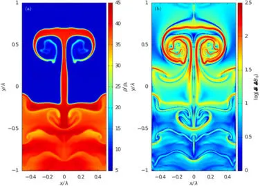
Rayleigh–Taylor and Richtmyer–Meshkov instabilities
Plateau–Rayleigh instability- The Plateau-Rayleigh Instability, often just called the Rayleigh instability, explains why and how a falling stream of fluid breaks up into smaller packets with the same volume but less surface area.
It is related to the Rayleigh Taylor Instability and is part of a greater branch of fluid dynamics concerned with fluid thread breakup. This fluid instability is exploited in the design of a particular type of ink jet technology whereby a jet of liquid is perturbed into a steady stream of droplets.


Now we are ready to perfom our Rayleigh Taylor Instability simulation. We devide our simulation in two cases. In case_1, we take air and water and here I perform three simulation in different mesh size.
CASE_1:- We devide our simulation in three part-
- Preprocessing and Mesh
- Case Setup
- Postprocessing Result
Preprocessing and Mesh:- At first geometry is created as square boxes and converted to surfaces using pull tool in Spaceclaim. And I turned on share topology to share the one edge between air and water.
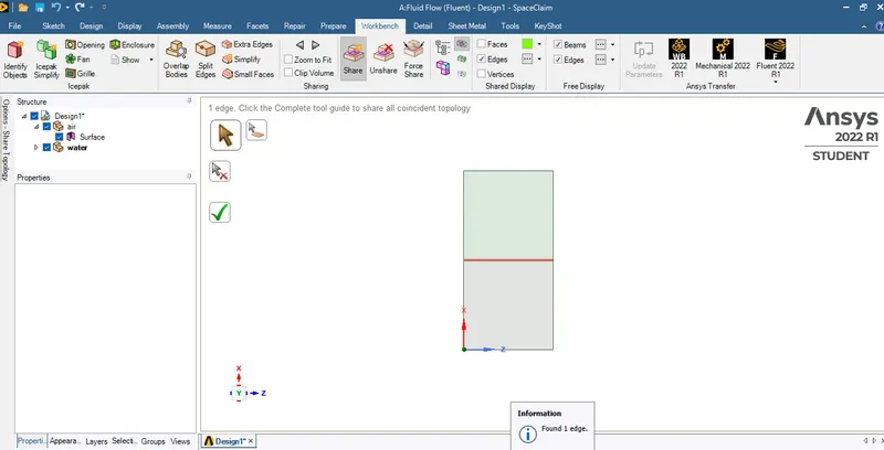
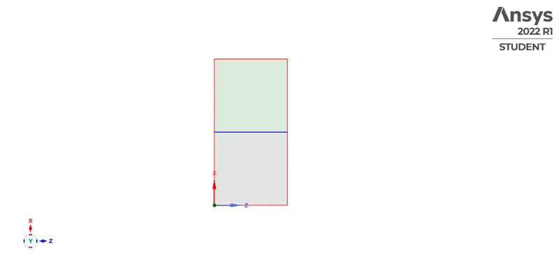
So, our geometry is now ready to go for meshing. We take base mesh size as 0.5
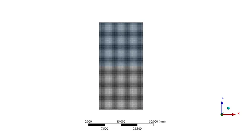
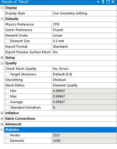
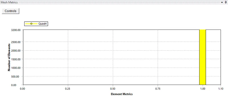
mesh details and quality check for 0.5 mm-
Then we take mesh size as 0.25mm
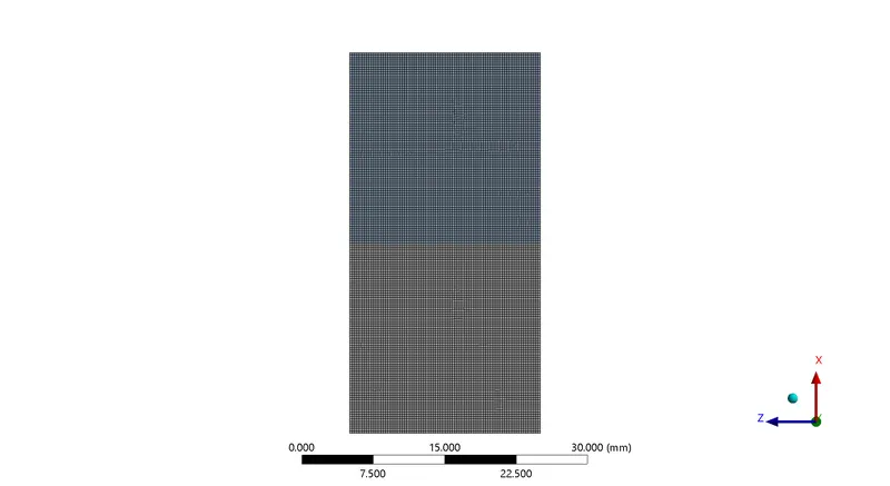
mesh details and quality check for 0.25 mm-
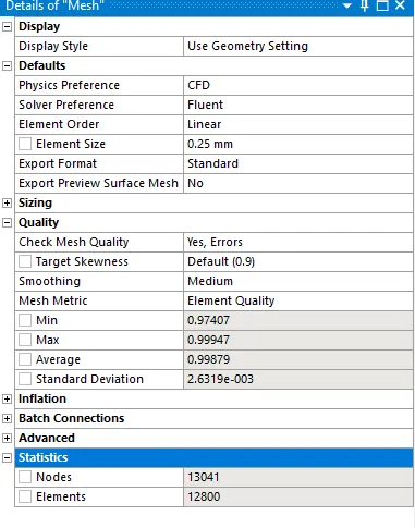
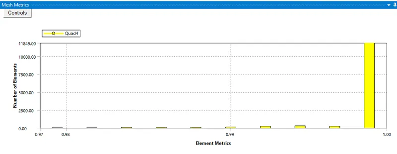
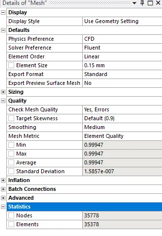
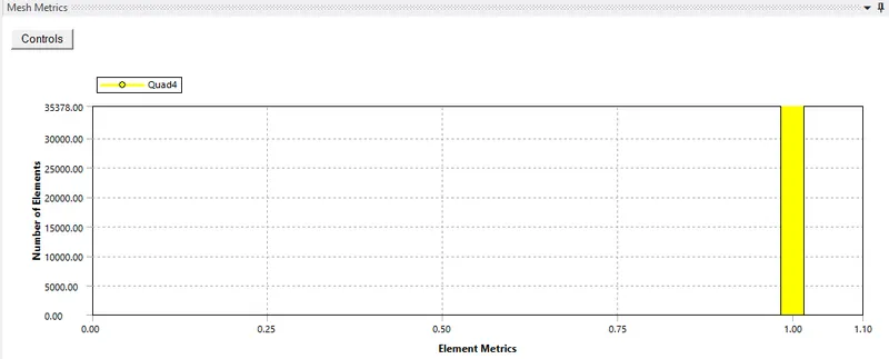
At last we take mesh size as 0.15 mm-
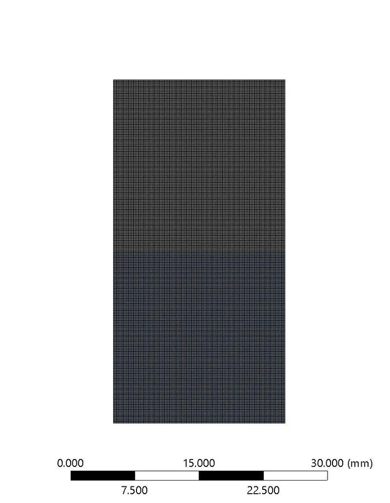
mesh details and quality check for 0.15 mm-
Case Setup and Solving:-
- Pressure-based solver and Absolute velocity are used.
- Transient-state Calculation is performed.
- Compressible fluid flow is chosen.
- Gravity is enabled in -ve Y-axis
- Multiphase Model is turned on along with Volume of Fluid and number of Eulerian phases is chosen as 2 and Implicit scheme is selected
- Viscous model-Laminar is used.
- Cell zone selected as Fluid-air;water-surface:water-liquid
- Patching of the volume fraction of the two phases is performed before the start of the simulation. The phase used for patching was water and a volume fraction of 1 is taken for water surface and 0 for air surface.
- In Pressure velocity coupling, a SIMPLE scheme is used. For the momentum, a second-order upwind scheme is used and for pressure, PRESTO is selected. For the transient formulation, a first-order implicit scheme is chosen for better results and stability and convergence of the residual
Report-
Fluent
Version: 2d, dp, pbns, vof, lam, transient (2d, double precision, pressure-based, VOF, laminar, transient)
Release: 22.1.0
Title:

Models
------

   Model                        Settings
   ---------------------------------------------------------
   Space                        2D
   Time                         Unsteady, 1st-Order Implicit
   Viscous                      Laminar
   Heat Transfer                Disabled
   Solidification and Melting   Disabled
   Species                      Disabled
   Coupled Dispersed Phase      Disabled
   NOx Pollutants               Disabled
   SOx Pollutants               Disabled
   Soot                         Disabled
   Mercury Pollutants           Disabled
   Structure                    Disabled
   Acoustics                    Disabled
   Eulerian Wall Film           Disabled
   Potential/Li-ion Battery     Disabled
   Multiphase                   Volume of Fluid


Material Properties
-------------------

   Material: water-liquid (fluid)

      Property                        Units      Method     Value(s)
      --------------------------------------------------------------
      Density                         kg/m^3     constant   998.2
      Cp (Specific Heat)              J/(kg K)   constant   4182
      Thermal Conductivity            W/(m K)    constant   0.6
      Viscosity                       kg/(m s)   constant   0.001003
      Molecular Weight                kg/kmol    constant   18.0152
      Thermal Expansion Coefficient   K^-1       constant   0
      Speed of Sound                  m/s        none       #f

   Material: air (fluid)

      Property                        Units      Method     Value(s)
      ----------------------------------------------------------------
      Density                         kg/m^3     constant   1.225
      Cp (Specific Heat)              J/(kg K)   constant   1006.43
      Thermal Conductivity            W/(m K)    constant   0.0242
      Viscosity                       kg/(m s)   constant   1.7894e-05
      Molecular Weight                kg/kmol    constant   28.966
      Thermal Expansion Coefficient   K^-1       constant   0
      Speed of Sound                  m/s        none       #f

   Material: aluminum (solid)

      Property               Units      Method     Value(s)
      -----------------------------------------------------
      Density                kg/m^3     constant   2719
      Cp (Specific Heat)     J/(kg K)   constant   871
      Thermal Conductivity   W/(m K)    constant   202.4


Cell Zone Conditions
--------------------

   Zones

      name                          id   type
      ----------------------------------------
      fff-air_surface (mixture)     3    fluid
      fff-air_surface (air)         3    fluid
      fff-air_surface (water)       3    fluid
      fff-water_surface (mixture)   4    fluid
      fff-water_surface (air)       4    fluid
      fff-water_surface (water)     4    fluid

   Setup Conditions

      fff-air_surface (mixture)

         Condition       Value
         ---------------------
         Frame Motion?   no
         Mesh Motion?    no

      fff-air_surface (air)

         Condition   Value
         -----------------

      fff-air_surface (water)

         Condition   Value
         -----------------

      fff-water_surface (mixture)

         Condition       Value
         ---------------------
         Frame Motion?   no
         Mesh Motion?    no

      fff-water_surface (air)

         Condition   Value
         -----------------

      fff-water_surface (water)

         Condition   Value
         -----------------


Boundary Conditions
-------------------

   Zones

      name                               id   type
      --------------------------------------------
      wall-fff-air_surface (mixture)     7    wall
      wall-fff-air_surface (air)         7    wall
      wall-fff-air_surface (water)       7    wall
      wall-fff-water_surface (mixture)   9    wall
      wall-fff-water_surface (air)       9    wall
      wall-fff-water_surface (water)     9    wall

   Setup Conditions

      wall-fff-air_surface (mixture)

         Condition                  Value
         ------------------------------------------
         Wall Motion                Stationary Wall
         Shear Boundary Condition   No Slip

      wall-fff-air_surface (air)

         Condition   Value
         -----------------

      wall-fff-air_surface (water)

         Condition   Value
         -----------------

      wall-fff-water_surface (mixture)

         Condition                  Value
         ------------------------------------------
         Wall Motion                Stationary Wall
         Shear Boundary Condition   No Slip

      wall-fff-water_surface (air)

         Condition   Value
         -----------------

      wall-fff-water_surface (water)

         Condition   Value
         -----------------


Solver Settings
---------------

   Equations

      Equation          Solved
      ------------------------
      Flow              yes
      Volume Fraction   yes

   Numerics

      Numeric                         Enabled
      ---------------------------------------
      Absolute Velocity Formulation   yes

   Unsteady Calculation Parameters


      --------------------------------
      Number of Time Steps       750
      Time Step Size [s]         0.005
      Max Iterations/Time Step   20

   Under-Relaxation Factors

      Variable          Relaxation Factor
      -----------------------------------
      Pressure          0.3
      Density           1
      Body Forces       1
      Momentum          0.7
      Volume Fraction   0.5

   Linear Solver

      Variable          Solver Type   Termination Criterion   Residual Reduction Tolerance
      ------------------------------------------------------------------------------------
      Pressure          V-Cycle       0.1
      X-Momentum        Flexible      0.1                     0.7
      Y-Momentum        Flexible      0.1                     0.7
      Volume Fraction   Flexible      0.1                     0.7

   Pressure-Velocity Coupling

      Parameter   Value
      ------------------
      Type        SIMPLE

   Discretization Scheme

      Variable          Scheme
      -------------------------------------
      Pressure          PRESTO!
      Momentum          Second Order Upwind
      Volume Fraction   Compressive

   Solution Limits

      Quantity                    Limit
      ---------------------------------
      Minimum Absolute Pressure   1
      Maximum Absolute Pressure   5e+10
      Minimum Temperature         1
      Maximum Temperature         5000
Postprocessing Result:- We run this case for 750 iterations and the time step size is 0.005.
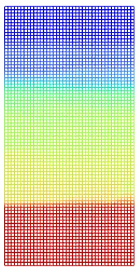
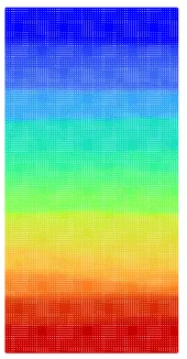
Comparing the result between three mesh size 0.5, 0.25 and 0.15 respectively.
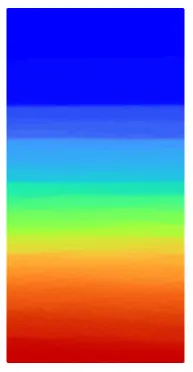
Rayleigh Taylor instability animation vedio for mesh size 0.5
Rayleigh Taylor instability animation vedio for mesh size 0.25
Rayleigh Taylor instability animation vedio for mesh size 0.15
The effect of mesh size on simulation:-
At first, the fluids behave linearly and we can observe small linearly sinking going on between them, slowly the chunky bubbles from the higher density fluid on top settle down. This can be identified from the highest mesh case resulting in the finest behavior of the instability for this condition. At t = 0, the small enough, initial perturbation in flow can be described by a smooth function. We observe the disturbance in flow from smooth to turbulent growth has been observed. We also observed the transition of a single globule into lots of deformed globules with lots of turbulence along with some breakup and penetration of heavier fluid into the lighter one, showing the phenomena of Rayleigh-Taylor instability.
For t<= 0.1, we observe a broadening of the interface as the diffusion takes place. For t>=1.5, the simulation enters the non-linear regime with the increase in the amplitude of perturbation. At the latter time, we observe the formation of low-density bubbles and their rise into the high-density phase whereas the high-density globules sink at the edge of the domain of the simulation into the lighter fluid. With the time evaluation, the interface gets smeared due to numerical diffusion within the interfaces. And the globules' shape deforms as the flow time increases and it also varies with the meshing. The volume fraction in simulation at a particular flow time shows the interface thickness is smaller on a finer mesh.
Why a steady-state approach might not be suitable for these types of simulation:-
Steady-state simulation computes the fully developed solution that does not change in time and Transient simulation computes the instantaneous values each time for each quantity. For Transient simulation, compared to steady-state, need more computational time. But, the Transient solver better captures the flow and can be used to run at smaller time steps which are seen in our case with a time step size of 0.005. Smaller time steps are required to observe the instabilities and can be only possible through transient simulation. Since it is a time marching solution, we expect more accuracy from transient simulation for which Transient simulation is the ideal setup to run the calculation for Rayleigh Taylor Instability.
CASE_2:-
We run one more simulation with water and user-defined material(density = 400 kg/m3, viscosity = 0.001 kg/m-s) for refined mesh. Here all the geometry and processes are same. So, we just focus on our result.
Postprocessing Result:- We run this case for 1500 iterations and the time step size is 0.005 to get a stable result.
Contour plot-
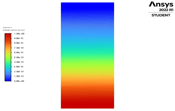
RT instability animation vedio-
ATWOOD NUMBER:- Atwood number is a dimensionless number in fluid mechanics used in the study of hydrodynamic instabilities in density-stratified flows.
A = `(rho_2 - rho_1)/(rho_2 + rho_1)`
Where, `rho_2` is the fluid density of heavier fluid
and `rho_1` is the fluid density of lighter fluid
In our case_1, water density is 998.2 kg/m^3, and air density is 1.225 kg/m^3. So, the Atwood number is-
A = `(998.2 - 1.225)/(998.2 + 1.225)` = 0.99
In our case_2, water density is 998.2 kg/m^3, and user-defined material density is 400 kg/m^3. So, the Atwood number is-
A = `(998.2 - 400)/(998.2 + 400)` = 0.42
In lower Atwood numbers, spikes and globules were still present at the end of the simulation which were not there in the Atwood Number of 0.9 in Case 1. With the increased Atwood Number close to 1 the stabilization effect of initial density stratification decreases and the instability caused by the expansion-compression effect becomes more significant.
It can be seen in the figures that the larger Atwood numbers, the larger amplitude of perturbation. It takes place due to the larger the density ratio of two fluids, the stronger force to develop the interface instability. The flow structure of bubbles and globules are quite different both for the variation in meshing and also for the variation in Atwood Number. With the increase of Atwood number, the time of spikes or globules of the lighter phase fluid arriving at the bottom of the computational domain is accelerated, then the duration of RTI in the steady growth stage is shorter. That's why in the case of 0.9 Atwood number, we get the same result but in 750 iterations, whereas in the case of 0.4 Atwood number we get that result after running 1500 iterations.
CONCLUSION:-
- For our simulation, the classical method of Finite Element analysis was adopted to study the evolution of the interface during RTI.
- The governing equations were Navier-Stokes equations and Cahn-Hilliard equations and the initial displacement disturbance was defined by the Cosine function.
- Transient simulation is the ideal setup to run the calculation for RT Instability.
- From the grid dependency test, we can observe that the interface thickness reduces with the refined mesh and when run with smaller time steps.
- With the increase of Atwood number, the time of spikes or globules of the lighter phase fluid arriving at the bottom of the computational domain is accelerated, then the duration of RTI in the steady growth stage is shorter. That's why we take higher iteration value for lower Atwood number.