Week 5 - Rayleigh Taylor Instability

1.Aim:

• To conduct the Rayleigh Taylor CFD simulation.

2.Introduction

• The Rayleigh–Taylor instability is an instability of an interface between two fluids of different densities which occurs when the lighter fluid is pushing the heavier fluid.
• A heavy fluid supported against gravity by a lighter fluid constitutes an unstable situation. A glass of water that is held inverted will cause the water to fall out the sides of the container, while a column of air rises along the center in its place. While the atmospheric pressure associated with the air column is sufficient to support the weight of the water, the instability is caused by tiny perturbations at the interface. More generally, the acceleration may be different from the earth’s gravity, or even impulsive where the resulting flow is called a RT instability.
• Examples:

1. Supernova explosion
2. Water suspended atop oil
3. Clouds formed due to volcanic eruptions
4. Atmosphere and etc.

3.CFD models that have been based on the mathematical analysis of Rayleigh Taylor waves.

3.1 Mass diffusion model:

• The mass diffusion equation describes the transport of mass and energy due to model viscosity and hence drives actual mixing in the fluids.Even if any configuration is Rayleigh-Taylor unstable, the diffusion process could be responsible for significsnt mixing if the viscosity is sufficiently large.

3.2 Single fluid model:

3.2.1 Potential flow model:

• The model is valid for all instabillity changes from the linear stage through the early non-linear to the asymptotic but limited to Atwood number = 1. In this model, single-mode peturbation expands the flow equations to second-order around the bubble tips, hence obtaining an ordinary differential equation for the bubble velocity.

3.2.1 Buoyancy drag model:

• It is valid for every Atwood number but limited to the non-linear stages of the instability. It uses ordinary differential equations to evolve the width of the mixing layer. The bubble, or spike, amplitudes are discribed by balancing the interia, buoyancy and drag forces.
• These models cannot model multiple mixing interfaces; cannot be easily extended to 2 or 3 dimensions, and as a rule, do not adress demixing, also known as counter gradient transport

3.2.3 Besnard-Harlow-Rauenzahn(BHR)

• It is a more advanced version of the single fluid model. The BHR model is based upon the evolution equations arising from second-order correlations and gradient-diffusion approximations. Using a mass-weighted averaged decomposition, the original BHR model includes full transport equations for the Reynold stresses, turbulent mass-flux velocity, density fluctuation and the turbulent kinetic energy dissipation rate.

3.3 Multi Fluid model:

• These models use a separate set of equations for each fluid in addition to the main flow equations and provide an accurate modeling framework for demixing by correctly capturing the relative motion of the different fluid fragments.
• The first step for the development of turbulence models is to perform Reynold averaging of the governing equations and resultant terms.

3.3.1 Two equation K-L turbulence model:

• The K-L turbulence model involves equations for turbulent kinematic energy K and turbulent length scale L. The starting point for deriving the model equations are the buoyancy-drag models for the self-similar growth of RT instabilities.

3.3.2 Three equation K-L-a turbulence model:

• The three equation model was developed as an extension to the two-equation K-L model by including a third equation for the turbulent mass-flux velocity.

3.3.3 Four equation K-L-a-b turbulence model:

• The four equation model was developed as an extension to the three-equation K-L model by including a fourth equation for density specific volume covariance. The model can accurately reflect the effects of the changes in the density fluctuations.

3.4 Steps involves in Ansys Fluent software

1. Geometry: Construct a two or three dimensional representation of the object to be modelled and tested using the work plane co-ordinate system within Ansys.
2. Mesh: At this point understands the makeup of the part. Now define how the modelled system should be broken down into finite pieces.
3. Setup: This case setup will be done using Ansys Fluent.
4. Solution: Ansys Fluent where run time result visualization is done.
5. Results: Post processing of results will be done using CFD post.

4.Procdure:

4.1 Geomentry

1.Open new project, by clicking on Fluid flow(Fluent) in Ansys workbench.

2.Now click on geometry to Draw a geometry. It will redirect to Spaceclaim, Ansys geometry model.

3Create square of a dimensions of 20mm.

4.And use pull tool to create a volume of air and create a new component as well same for water volume.

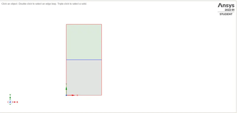
5. Now select the share topology, One edge can be shared.

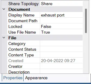
Fig: Share Topology

4.2 Mesh

6.Select wall face and press right click of mouse, it will open a menu. Click on option create named selection and write suitable name for faces.

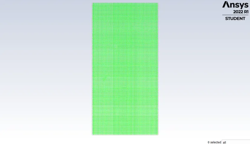
7. Now click on mesh option and choose generate mesh. It will generate mesh Initial mesh.

8. Now change the quality of mesh for getting finer mesh.

4.3 Setup and Solution

9.Exit mesh and open setup. First, Check mesh, it is throwing no error then only we can proceed further. We are going to do pressure based Transient state simulation and Gravity -9.81 in Y direction, So choose these options on task page.

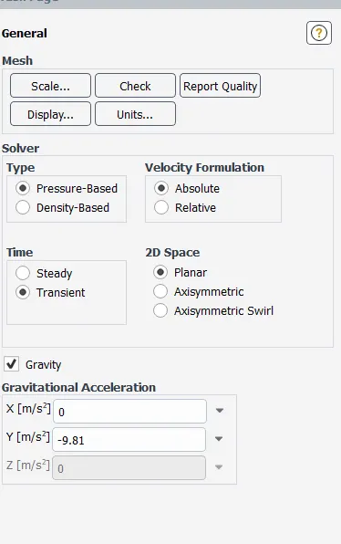
Fig: Task page

10. Go to physics menu and select viscous model. It will open a menu, choose realizable Laminer flow.

11. Select multiphase and select the volume and implicit Method.

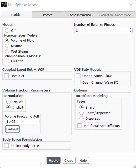
Fig: Multiphase

12. Move to phase and choose a primary and secondary phases of materials.

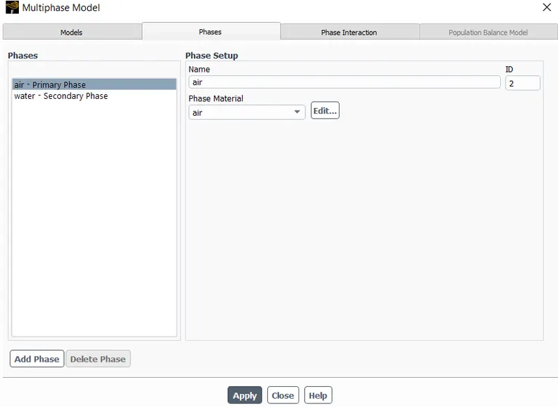
Fig: Phase selection

12.Click on material and choose air as working fluid. check working fluid by clicking on cell zone conditions option, if it Fluid is air & water then proceed.

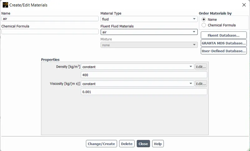
Fig: 1st Mateials

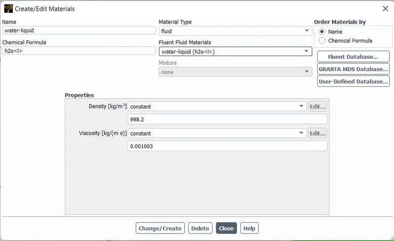
Fig: 2nd materials

12.Now click on intialization to calculate approximate values of velocity and pressure.

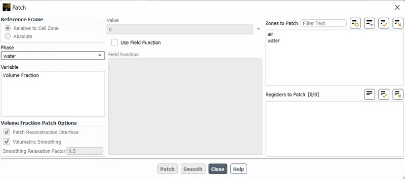
Fig: Selecting patch

13.Change the number of iteration and Time step

Time step size = (Flow time/Time step)

14.Exit setup and double click on result to open CFD post. Check boxes to see walls and other parts.

5.Results:

5.1 Atwood number:

It is a dimensionless number that is used to study hydrodynamic instabilities in density stratified flows.

A=(ρ1-ρ2)/(ρ1+ρ2)

Where,

ρ1 is density of heavier fluid

ρ2 is density of lighter fluid

For Air-Water RT instability

ρ1=998.2 kg/m^3 (water density)

ρ2=1.225 kg/m^3 (air density)

A=(998.2-1.225)/(998.2+1.225)

A=0.998

For User Defind material-Water RT instability

ρ1=998.2 kg/m^3 (water density)

ρ2=400 kg/m^3 (UD density)

A=(998.2-400)/(998.2+400)

A=0.428

Output for Air-Water RT instability

Residual

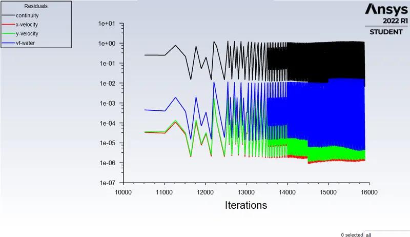
Output for user defind material-Water RT instability

5.2 Observation:

• Finer mesh captures the instability better than the coarse mesh, but it takes more time for the heavier fluid to settle down. So it is computationally expensive but produces results with better accuracy.
• The simulation involves capturing instabilities which are changing in an unpredictable manner as a function of time, transient approach is preferred over steady state approach.

6.Conclusion:

• Atwood number forms a basis to compare and study research paper based on RT instability. Thus we can use these papers to validate our results for better accuracy.