Week 7 - Simulation of a 1D Super-sonic nozzle flow simulation using Macormack Method

AIM

Solve the conservation and non-conservation forms of the governing equations of 1D subsonic-supersonic nozzle by using MacCormack method.

Objective

1. Steady-state distribution of primitive variables inside the nozzle.
2. Time-wise variation of the primitive variables.
3. Variation of Mass flow rate distribution inside the nozzle at different time steps during the time-marching process.

Description

We consider the study, Isentropic flow through the nozzle, The flow through the nozzle inlet is from reservoir. The cross section area of nozzle is very large and hence the velocity is small. The flow locally subsonic the convergence section of the nozzle. sonic at the throat section and supersonic at the divergent section.

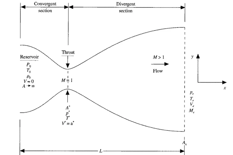
Let as consider a small control volume of the nozzle as shown below

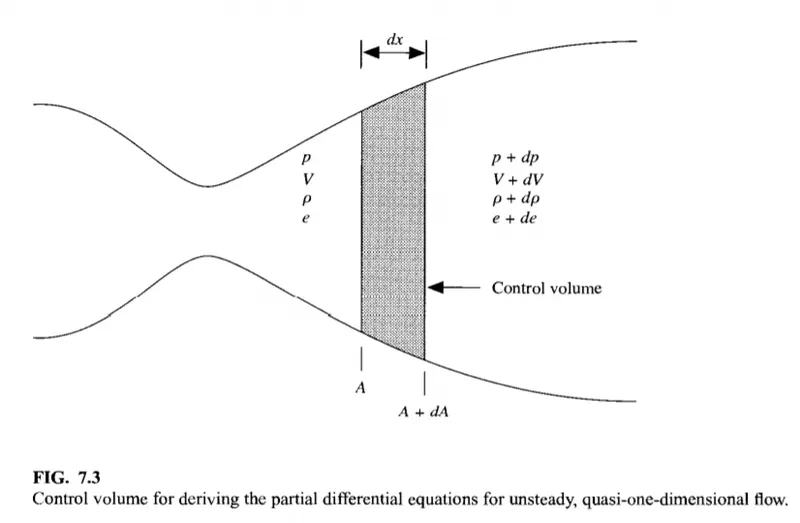
We assume that at a given section, where the cross section, where the cross section area is A,the flow properties are uniform across the section.Hence although the area of the nozzle changes as a function of distance along the nozzle.X, and therefore in reality the flow field is two dimensional. we make the assumption that the flow properties vary only with X; this is that amount to assume uniform flow properties across any given cross-section. such flow is defind as Quasi one dimensional flow.

The governing continuty, momentum and energy equation in terms of non dimentional variable for this quasi one dimensional steady and isentropic flow can be expressed respectively,

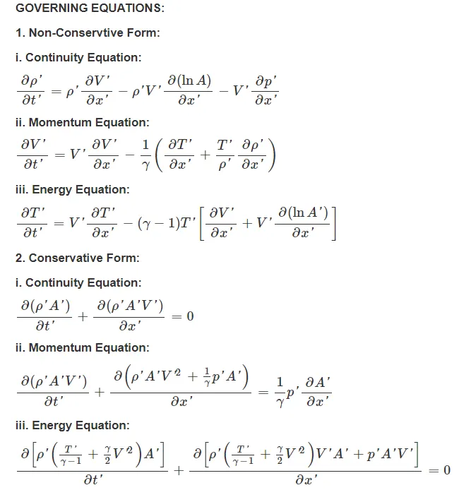
This equation are macomark method using the time marching process

The MacCormack method is a variation of the two step Lax-Wendroff scheme but is much simpler in application. To illustrate the algorithm, consider the following first order hyperbolic equation

The application of MacCormack method to the above equation proceeds in two steps; a predictor step which is followed by a corrector step.

Predictor step: In the predictor step, a "provisional" value of u at time level n+1 (denoted by ) is estimated as follows

The above equation is obtained by replacing the spatial and temporal derivatives in the previous first order hyperbolic equation using forward differences.

Corrector step: In the corrector step, the predicted value is corrected according to the equation

Note that the corrector step uses backward finite difference approximations for spatial derivative. The time-step used in the corrector step is in contrast to the used in the predictor step.

Replacing the term by the temporal average

to obtain the corrector step as

Calculation of Time-step

In order for the solution to be stable, the concept of courant flow number was introduced in previous projects. forna linear hyperbolic equation, the value CFL<1 will give a stable solution.

For this project CFL=0.5 and value of time step is calculated as follows △t=c*(△x/(v+a))

where, c is courant number, v is local flow velocity at a point and a is the local speed of sound. value of dt at all grid points is calculated and the minimum of them is chosen for the simulation.

Boundary condition

At the inlet

Velocity at the inlet is changing with time,while the density and temperature are constant with respect to time

u1 = 2u2+u3

velocity at the inlet is calculated by the method of linear extrapolation. values of velocity at node 2 and 3 are used for the same.

At the oulet

All the variables at the outlet are kept changing with respect to time and linear extrapolation is used to calculated the variable at the outlet.

v(n)=2*v(n-1)-v(n-2);
rho(n)=2*rho(n-1)-rho(n-2);
t(n)=2*t(n-1)-t(n-2);

Initial condition

Area of the nozzle will remain constant throughout the time simulation

a=1+(2.2*((x-1.5).^2))

The flow-field variable vary with respect to time. At t=0, their values are given as

rho=1-(0.3146*x);
t=1-(0.2314*x);
v=(0.1+1.09*x).*t.^0.5;

Conservation Form

The governing equation are expressed in a generic form which consists of the solution vector U, the flux vector F and the source term J.

(∂U/∂t)+(∂F/∂x) =J

The equation for Quasi 1D supersonic flow can be expressed in a similar generic form as follows

u1=ρ.*a;
u2=ρ.*a.*v;
u3=ρ.*a.*((t./(γ-1))+((γ/2)*(v.^2)));

The equation solved using maccmark method.

f1=u2;
f2=((u2.^2)./u1)+(((γ-1)/γ)*(u3-((γ/2)*((u2.^2)./u1))));
f3=(γ*((u2.*u3)./u1))-(((γ*(γ-1))/2)*((u2.^3)./(u1.^2)));

Boundary condition

At the inlet

u2 and u3 are changing respective to time where as u1 is kept as constant

u1(1)=ρ(1)*a(1);
u2(1)=(2*u2(2))-u2(3);
u3(1)=u1(1)*((t(1)/(γ-1))+((γ/2)*(v(1)^2)));

At the Outlet

u1(n)=(2*u1(n-1))-u1(n-2);
u2(n)=(2*u2(n-1))-u2(n-2);
u3(n)=(2*u3(n-1))-u3(n-2);

Initial conditions

Area of the nozzle is constant throughout the runtime of simulation and its value is same as that taken for non-consevation form

Initial velocity is given as, u=(0.59/ρ*a)

At t=0, values of density and temperature throughout the nozzle are given as follows,

(x(c)<=0.5)
ρ(c)=1;
t(c)=1;
(x(c)>0.5) && (x(c)<=1.5)
ρ(c)=1-(0.366*(x(c)-0.5));
t(c)=1-(0.167*(x(c)-0.5));
ρ(c)=(0.634-(0.3879*(x(c)-1.5)));
t(c)=(0.833-(0.3507*(x(c)-1.5)));

Main code for Non-Conservation form

clear all
close all
clc
% inputs 
n=31;
x=linspace(0,3,n);
dx= x(2)-x(1);
gamma=1.4;
%calculate initial profile
rho=1-(0.3146*x);
t=1-(0.2314*x); % t = temperature
v=(0.1+1.09*x).*t.^0.5;
 %area
a=1+(2.2*((x-1.5).^2));
%courant number
c=0.5;
%finding the throat grid point
thr=find(a==1);
%for loop to determine the dt values at each value
for m=1:n
    dt_grid(m)=c*(dx/((t(m))^0.5+v(m)));
end
% number time step
nt=1400;
dt=min(dt_grid);
tic
%outer time loop
for k= 1:nt
   rho_old = rho;
   v_old = v;
   t_old = t;
   %predictor method
   for j=2:n-1
       %drho_dt_p = -((rho(j)*(v(j+1)-v(j))/dx)-(rho(j)*v(j)*(log(a(j+1)-log(a(j))))/dx)-(v(j)*(rho(j+1)-rho(j))/dx));
    dvdx=(v(j+1)-v(j))/dx;
    drhodx=((rho(j+1)-rho(j)))/dx;
    dtdx=(t(j+1)-t(j))/dx;
    dlogadx=(log(a(j+1))-log(a(j)))/dx;
   %continunity equation
   drho_dt_p(j) = -rho(j)*dvdx-rho(j)*v(j)*dlogadx-v(j)*drhodx;
   %momentum equation
   dvdt_p(j)=-v(j)*dvdx-(1/gamma)*(dtdx+(t(j)/rho(j))*drhodx);
   %energy equation
   dtdt_p(j)=-v(j)*dtdx-((gamma-1)*t(j)*((dvdx)+v(j)*dlogadx));
      %solution update
       rho(j)=rho(j)+(drho_dt_p(j))*dt;
       v(j)=v(j)+dvdt_p(j)*dt;
       t(j)=t(j)+dtdt_p(j)*dt;
   end

  
 %Corrector method
   for j=2:n-1
       %drho_dt_p = -((rho(j)*(v(j+1)-v(j))/dx)-(rho(j)*v(j)*(log(a(j+1)-log(a(j))))/dx)-(v(j)*(rho(j+1)-rho(j))/dx));
    dvdx=(v(j)-v(j-1))/dx;
    drhodx=((rho(j)-rho(j-1)))/dx;
    dtdx=(t(j)-t(j-1))/dx;
    dlogadx=(log(a(j))-log(a(j-1)))/dx;
   %continunity equation
   drho_dt_c(j)= -rho(j)*dvdx-rho(j)*v(j)*dlogadx-v(j)*drhodx;
   %momentum equation
   dvdt_c(j) = -v(j)*dvdx-(1/gamma)*(dtdx+(t(j)/rho(j))*drhodx);
   %energy equation
   dtdt_c(j) = -v(j)*dtdx-((gamma-1)*t(j)*((dvdx)+v(j)*dlogadx));
         %solution update
       rho(j)=rho(j)+(drho_dt_p(j))*dt;
       v(j)=v(j)+dvdt_p(j)*dt;
       t(j)=t(j)+dtdt_p(j)*dt;
   end
   %final solution updates
  for i=2:n-1
   %computate the range of derivatives
   drhodt(i) = 0.5*(drho_dt_p(i)+drho_dt_c(i));
   dvdt(i)= 0.5*(dvdt_p(i)+dvdt_c(i));
   dtdt(i)= 0.5*(dtdt_p(i)+dtdt_c(i));
   % final solution update 
       rho(i)=rho_old(i)+drhodt(i)*dt;  
       v(i)=v_old(i)+dvdt(i)*dt; 
       t(i)=t_old(i)+dtdt(i)*dt;
   end
   % Apply boundary condition
   %inlet boundary condition
   v(1)=2*v(2)-v(3);
   %outlet boundary condition
   v(n)=2*v(n-1)-v(n-2);
   rho(n)=2*rho(n-1)-rho(n-2);
   t(n)=2*t(n-1)-t(n-2);
  % calculating the variables such mac number,pressure
    %pressure ratio
    pr=rho.*t;
    %mac number
    mac=v./(t.^0.5);
    %mass flow rate
    mass_flow=rho.*v.*a;
  %field variables at throat section
  rho_thr(k)=rho(thr);
  t_thr(k)=t(thr);
  pr_thr(k)=pr(thr);
  mac_thr(k)=mac (thr);
  mass_flow_thr(k)=mass_flow(thr);
  %Throat section residual values
  rho_res(k)=drhodt(thr);
  t_res(k)=dtdt(thr);
  v_res(k)=dvdt(thr);
  %plotting the mass flow rate at different time
  plot_mass_flow_rate(x,mass_flow,k)
  %plotting the field variables
  plot_field_variable(x,pr,rho,t,mac,k)
end
 plot_fieldvar_throat(rho_thr,pr_thr,t_thr,mac_thr)
 plot_vaiables_residual(rho_res,t_res,v_res)
 time=toc;
sprintf('time taken for execution is %f',time)

Explanation

• Code is started with clear all, close all, and clc to enable a fresh start without the manipulation of previous values.
• Input parameters are assigned for the variable x,dx,n,gamma,nt and c.
• tic toc command is used for calculating the time elapsed between code.
• For initial boundary conditions are established for density.
• Now outer time loop is computed for for loop to calculate all the grid point for various formulas inside the loop.
• MacCarmack technique is used to solve the numerical solution of governing equation such as Continunity, Momentum & Energy equation
• The technique implies two method s for solving namely predictor method followed by corrector method.
• perdictor & corrector methods are assigned within the for loop individually for calculating values.
• The calculated values are averaged in the next step and updating the solution with old values.
• Boundary conditions are applied within the for loop and subsequently used for calculating the mass flow rate, mach number and pressure and also calculating the values throat section.
• program is ended.

Function code for Mass flow rate

function []=plot_mass_flow_rate(x,mass_flow,k)
figure(1)
if (k==1)
    plot(x,mass_flow,'m')
    xlabel('nozzle domain')
    ylabel('mass flow rate')
    title('mass flow rate along length of nozzle')
    hold on
elseif (k==101)
    loglog(x,mass_flow,'g')
    hold on
elseif (k==201)
    loglog(x,mass_flow,'r')
    hold on
elseif (k==601)
    loglog(x,mass_flow,'y')
    hold on
elseif (k==801)
    loglog(x,mass_flow,'b')
    hold on
    legend('k1','k101','k201','k601','k801')

end
end

Function code for ploting the variable

function []=plot_field_variable(x,pr,rho,t,mac,k)
    figure(2)
    subplot(4,1,1)
    plot(x,pr)
    xlabel('nozzle domain')
    ylabel('pressure')
    title(sprintf('variation of pressure along the length of the domain and itr is %d',k))
    axis([0.5 3 0 max(pr)])

    subplot(4,1,2)
    plot(x,rho)
    xlabel('nozzle domain')
    ylabel('density')
    title(sprintf('variation of density along the length of the domain and itr is %d',k))
    axis([0.5 3 0 max(rho)])

    subplot(4,1,3)
    plot(x,t)
    xlabel('nozzle domain')
    ylabel('temperature')
    title(sprintf('variation of temperature  along the length of the domain and itr is %d',k))
    axis([0.5 3 0 max(t)])

    subplot(4,1,4)
    plot(x,mac)
    xlabel('nozzle domain')
    ylabel('mach number')
    title(sprintf('variation of mac number along the length of the domain and itr is %d',k))
    axis([0.5 3 0 5])
end

Function plot variable at throat section

function []=plot_fieldvar_throat(rho_thr,t_thr,mac_thr,pr_thr)
rho_ex = 0.634*ones(1,1400);
t_ex = 0.833*ones(1,1400);
mac_ex = ones(1,1400);
pr_ex = 0.579*ones(1,1400);

figure(3)
plot(rho_thr,'g')
hold on
plot(rho_ex)
xlabel('iteration')
ylabel('density')
title('density at throat')

figure(4)
plot(t_thr,'r')
hold on
plot(t_ex)
xlabel('iteration')
ylabel('temperature')
title('temperature at throat')

figure(5)
plot(mac_thr,'b')
hold on
plot(mac_ex)
xlabel('iteration')
ylabel('mac number')
title('mac number at throat')

figure(6)
plot(pr_thr,'y')
hold on
plot(pr_ex)
xlabel('iteration')
ylabel('pressure')
title('pressure at throat')
end

Function for plot residual values

function []=plot_vaiables_residual(rho_res,t_res,v_res)
%plot for residual
figure(7)
plot(rho_res)
hold on
plot(t_res,'r')
hold on
plot(v_res,'g')
xlabel('Number of iteration')
ylabel('Residual')
title('Residual at throat')
legend('rho_res','t_res','v_res','Location','best')
end

Explanation

• Separate functions for mass flow rate, the variable,variable at throat section and residual values
• Each plots have subplot for primitive variables such as Density, Pressure,Temperature and Mac number at throat section as well as convergent and divergent of the nozzle.

Result

1.Result for non conservation form

1.1 Variation of feild variables along the length of the nozzle

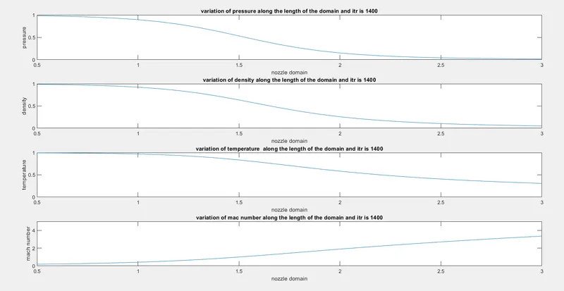
The above plot provides information regarding variation of flow variables along the length of the domain. Pressure, Density and Temperature decreases along the length of the domain, where as the Mac number increase the along the length of domain.

1.2 Mass flow rate along the length of the nozzle

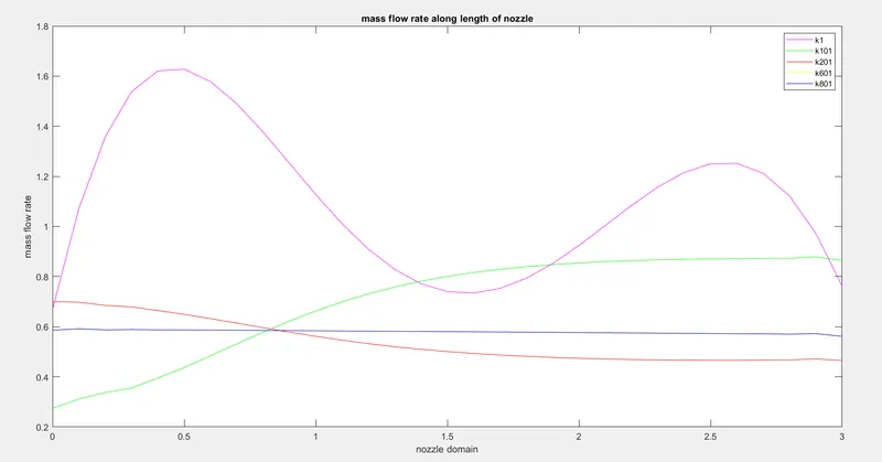
The above graph shows the mass flow rate at different time steps in the nozzle. After 600-700 time step, the mass flow rate is constant for any time step above 700 time step throughout the nozzle.

1.3 Temperature at throat

1.4 Pressure at throat

1.5 Density at throat

1.6 Mac number at throat

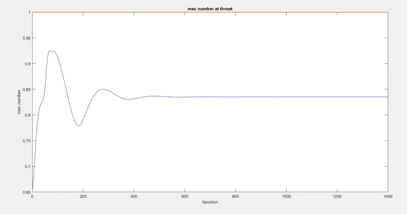
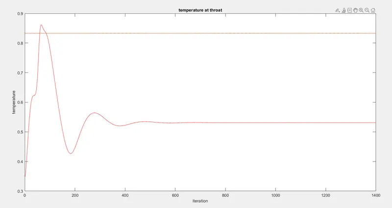
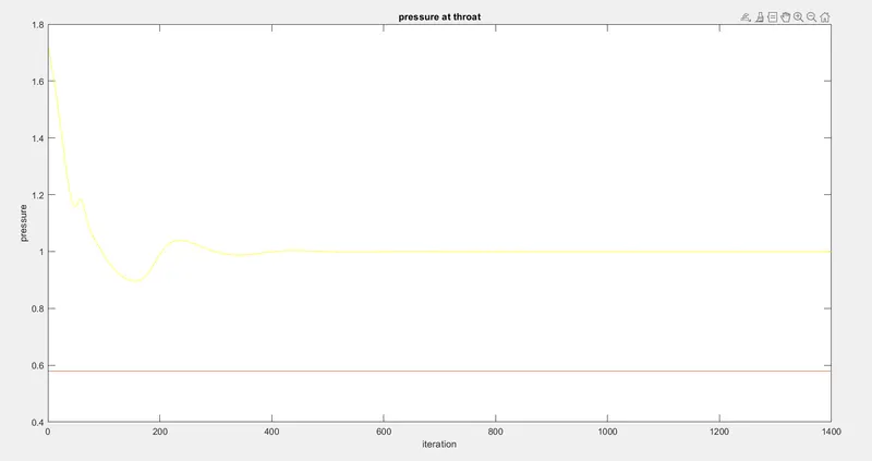
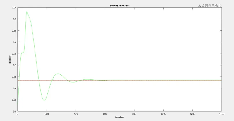
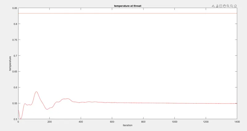
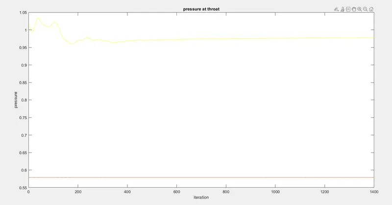
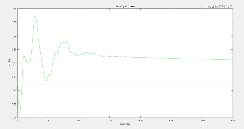
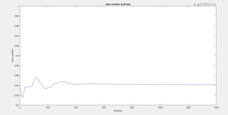
The above shows the variation of flow variables in the cross section of the throat for different iterations. It has been observed after 400 it solution is getting stability, but there is a small difference between exact and numerical solution.

1.7 Residual at throat

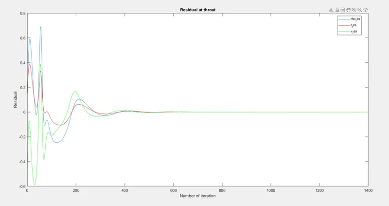
Main code for Conservation form

%conservation form 
clear all
close all
clc
% inputs 
n=31;
x=linspace(0,3,n);
dx= x(2)-x(1);
gamma=1.4;
%defining initial condition 
%defining density,temperature
for c=1:n
    if (x(c)<=0.5)
        rho(c)=1;
        t(c)=1;
    elseif (x(c)>0.5) && (x(c)<=1.5)
        rho(c)=1-(0.366*(x(c)-0.5));
        t(c)=1-(0.167*(x(c)-0.5));
    else 
        rho(c)=(0.634-(0.3879*(x(c)-1.5)));
        t(c)=(0.833-(0.3507*(x(c)-1.5)));
    end
end
%area 
a=1+(2.2*((x-1.5).^2));
%velocity
v=((0.59)./(rho.*a));
%defining the dt values
%courant number
c=0.5;
for m=1:n
    dt_grid(m)=c*(dx/(((t(m))^0.5)+(v(m))));
end
% number time step
nt=1400;
dt=min(dt_grid);
%defining the initial condition for solution vector
u1=rho.*a;
u2=rho.*a.*v;
u3=rho.*a.*((t./(gamma-1))+((gamma/2)*(v.^2)));
tic;
%finding the area at the grid point
thr=find(a==1);
%determing the parameter using the mac mark method
for k=1:nt
    u1_old=u1;
    u2_old=u2;
    u3_old=u3;
    %defining flux term
    f1=u2;
    f2=((u2.^2)./u1)+(((gamma-1)/gamma)*(u3-((gamma/2)*((u2.^2)./u1))));
    f3=(gamma*((u2.*u3)./u1))-(((gamma*(gamma-1))/2)*((u2.^3)./(u1.^2)));
    %predictor method
    for j=2:n-1
         j2(j)=(1/gamma)*rho(j)*t(j)*((a(j+1))-(a(j)))/dx;
         %solution vector
         du1dt_p(j)= -((f1(j+1)-f1(j))/dx);
         du2dt_p(j)= -((f2(j+1)-f2(j))/dx)+j2(j);
         du3dt_p(j)= -((f3(j+1)-f3(j))/dx);
         %update solution
         u1(j)=(du1dt_p(j)*dt)+u1(j);
         u2(j)=(du2dt_p(j)*dt)+u2(j);
         u3(j)=(du3dt_p(j)*dt)+u3(j);
    end
    %premitive value for corrector step
    rho=u1./a;
    v=u2./u1;
    t=(gamma-1)*((u3./u1)-((gamma/2)*(v.^2)));
    %defining flux value 
    F1=u2;
    F2=((u2.^2)./u1)+(((gamma-1)/gamma)*(u3-((gamma/2)*((u2.^2)./u1))));
    F3=(gamma*((u2.*u3)./u1))-(((gamma*(gamma-1))/2)*((u2.^3)./(u1.^2)));
    %corrector method
    for j=2:n-1
         j2(j)=(1/gamma)*rho(j)*t(j)*((a(j))-(a(j-1)))/dx;
         %solution vector
         du1dt_c(j)= -((F1(j)-F1(j-1))/dx);
         du2dt_c(j)= -((F2(j)-F2(j-1))/dx)+j2(j);
         du3dt_c(j)= -((F3(j)-F3(j-1))/dx);
    end
    %computing average value
    for i=2:n-1
        du1dt(i) = 0.5*(du1dt_p(i)+du1dt_c(i));
        du2dt(i)= 0.5*(du2dt_p(i)+du2dt_c(i));
        du3dt(i)= 0.5*(du3dt_p(i)+du3dt_c(i));
        % final solution update
        u1(i)=du1dt(i)*dt+u1_old(i);
        u2(i)=du2dt(i)*dt+u2_old(i);
        u3(i)=du3dt(i)*dt+u3_old(i);
    end
    %At boundary
    %Inlet
    u1(1)=rho(1)*a(1);
    u2(1)=(2*u2(2))-u2(3);
    u3(1)=u1(1)*((t(1)/(gamma-1))+((gamma/2)*(v(1)^2)));
    %Outlet
    u1(n)=(2*u1(n-1))-u1(n-2);
    u2(n)=(2*u2(n-1))-u2(n-2);
    u3(n)=(2*u3(n-1))-u3(n-2);
    % Decoding the solution vector
    rho=u1./a;
    v=u2./u1;
    t=(gamma-1)*((u3./u1)-((gamma/2)*(v.^2)));
     % calculating the variables such mac number,pressure
    %pressure ratio
    pr=rho.*t;
    %mac number
    mac=v./(t.^0.5);
    %mass flow rate
    mass_flow=rho.*v.*a;
  %field variables at throat section
  rho_thr(k)=rho(thr);
  t_thr(k)=t(thr);
  pr_thr(k)=pr(thr);
  mac_thr(k)=mac (thr);
  mass_flow_thr(k)=mass_flow(thr);
  %Throat section residual values
  u1_res(k)=du1dt(thr);
  u2_res(k)=du2dt(thr);
  u3_res(k)=du3dt(thr);
  %plotting the mass flow rate at different time
  plot_mass_flow_rate_c(x,mass_flow,k)
  %plotting the field variables
  plot_field_variable_c(x,pr,rho,t,mac,k)
end
 plot_fieldvar_throat_c(rho_thr,pr_thr,t_thr,mac_thr)
 plot_vaiables_residual_c(u1_res,u2_res,u3_res)
 time=toc;
sprintf('time taken for execution is %f',time)

Explanation

• Code is started with clear all, close all, and clc to enable a fresh start without the manipulation of previous values.
• Input parameters are assigned for the variable x,dx,n,gamma,nt and c.
• Initial value of area, throat, velocity, pressure are calculating using formula.
• In order to simplify and svoid the error, in equation is splitted into solution Vector, flux vector and source term.
• Now outer time loop is computed for for loop to calculate all the grid point for various formulas inside the loop.
• MacCarmack technique is used to solve the numerical solution of governing equation such as Continunity, Momentum & Energy equation
• The technique implies two method s for solving namely predictor method followed by corrector method.
• perdictor & corrector methods are assigned within the for loop individually for calculating values.
• The calculated values are averaged in the next step and updating the solution with old values.
• Boundary conditions are applied within the for loop and subsequently used for calculating the mass flow rate, mach number and pressure and also calculating the values throat section.
• program is ended.

Function code for Mass flow rate

function []=plot_mass_flow_rate_c(x,mass_flow,k)
figure(1)
if (k==1)
    plot(x,mass_flow,'m')
    xlabel('nozzle domain')
    ylabel('mass flow rate')
    title('mass flow rate along length of nozzle')
    hold on
elseif (k==101)
    loglog(x,mass_flow,'g')
    hold on
elseif (k==201)
    loglog(x,mass_flow,'r')
    hold on
elseif (k==601)
    loglog(x,mass_flow,'y')
    hold on
elseif (k==801)
    loglog(x,mass_flow,'b')
    hold on
    legend('k1','k101','k201','k601','k801')

end
end

Function code for ploting the variable

function []=plot_field_variable_c(x,pr,rho,t,mac,k)
    figure(2)
    subplot(4,1,1)
    plot(x,pr)
    xlabel('nozzle domain')
    ylabel('pressure')
    title(sprintf('variation of pressure along the length of the domain and itr is %d',k))
    axis([0.5 3 0 max(pr)])

    subplot(4,1,2)
    plot(x,rho)
    xlabel('nozzle domain')
    ylabel('density')
    title(sprintf('variation of density along the length of the domain and itr is %d',k))
    axis([0.5 3 0 max(rho)])

    subplot(4,1,3)
    plot(x,t)
    xlabel('nozzle domain')
    ylabel('temperature')
    title(sprintf('variation of temperature  along the length of the domain and itr is %d',k))
    axis([0.5 3 0 max(t)])

    subplot(4,1,4)
    plot(x,mac)
    xlabel('nozzle domain')
    ylabel('mach number')
    title(sprintf('variation of mac number along the length of the domain and itr is %d',k))
    axis([0.5 3 0 5])
end

Function plot variable at throat section

function []=plot_fieldvar_throat_c(rho_thr,t_thr,mac_thr,pr_thr)
rho_ex = 0.634*ones(1,1400);
t_ex = 0.833*ones(1,1400);
mac_ex = ones(1,1400);
pr_ex = 0.579*ones(1,1400);

figure(3)
plot(rho_thr,'g')
hold on
plot(rho_ex)
xlabel('iteration')
ylabel('density')
title('density at throat')

figure(4)
plot(t_thr,'r')
hold on
plot(t_ex)
xlabel('iteration')
ylabel('temperature')
title('temperature at throat')

figure(5)
plot(mac_thr,'b')
hold on
plot(mac_ex)
xlabel('iteration')

Function for plot residual values

function []=plot_vaiables_residual_c(u1_res,u2_res,u3_res)
%plot for residual
figure(7)
plot(u1_res)
hold on
plot(u2_res,'r')
hold on
plot(u3_res,'g')
xlabel('Number of iteration')
ylabel('Residual')
title('Residual at throat')
legend('u1','u2','u3','Location','best')
end

Explanation

• Separate functions for mass flow rate, the variable,variable at throat section and residual values
• Each plots have subplot for primitive variables such as Density, Pressure,Temperature and Mac number at throat section as well as convergent and divergent of the nozzle.

2.Result for conservation form

2.1 Variation of feild variables along the length of the nozzle

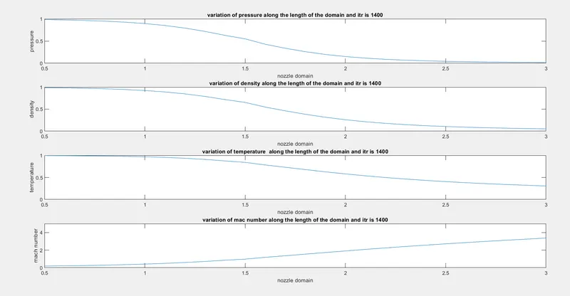
The above plot provides information regarding variation of flow variables along the length of the domain. Pressure, Density and Temperature decreases along the length of the domain, where as the Mac number increase the along the length of domain.For both forms, behaviour is same.

2.2 Mass flow rate along the length of the nozzle

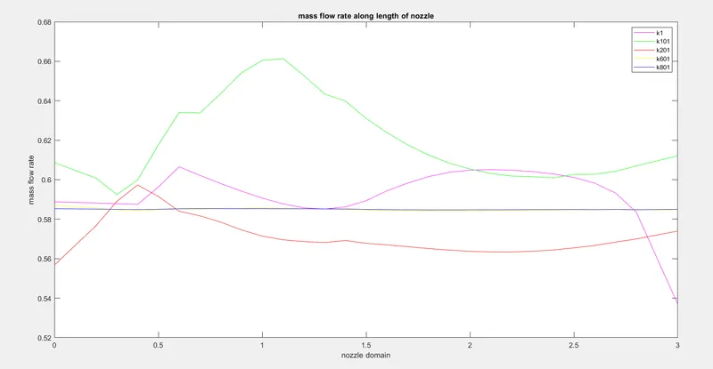
The above graph shows the mass flow rate at different time steps in the nozzle. After 600-700 time step, the mass flow rate is constant for any time step above 700 time step throughout the nozzle. when compared to non-conservation method fluctuation is less.

2.3 Temperature at throat

2.4 Pressure at throat

2.5 Density at throat

2.6 Mac number at throat

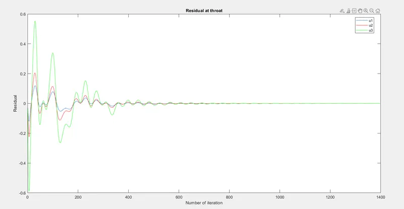
2.7 Residual at throat

Grid dependance test:

In order to conduct grid dependancy test, here two situation are considered one with 31 grid points and otherwise 61 Grid points. values here shown are from the grid where the throat area lies. From the below table it can be seen that the increase in grid point will increase the accuracy but the run of the simulation also drastically increase with the increase in the number of grid points. It means that faster result less is accuracy.

	T ratio	Pr ratio	Mach number	ρ ratio	Mass flow rate
Exact solution	0.833	0.528	1	0.634	0.579
Non conservation (31 gird point)	0.8365	0.5342	0.9994	0.6387	0.5838
Non conservation (61 gird point)	0.8354	0.5327	0.9998	0.6377	0.5827
conservation (31 gird point)	0.8406	0.5477	0.9795	0.6516	0.5852
conservation (61 gird point)	0.8353	0.5333	0.9989	0.6392	0.5829

Conclusion

1.After comparing both the methods it has been seen thet there are a lot more fluctuation in non-conservative flow when compared to the conservative one.

2.After comparing both the forms in terms of execution time non-conservation form is faster when compared to a conservative form. The main reason is the conservative part has more mathematical calculation.

3.Non-conservative form converages more quickly after 300 iteration solution starts converging where as conservative part requires 400 iteration.

4.Complexity in solving the conservative form is more when compared to non-conservative since the conservative part has more mathematical calculation when compared to other forms.