Week 5.1 - Mid term project - Solving the steady and unsteady 2D heat conduction problem

Aim:

     i) To Solve the 2D heat conduction equation by using the point iterative techniques.

    ii) To solve implicit iterative technique equations. 

                1. Jacobi

                2. Gauss-seidel

                3. Successive over-relaxation

   iii) To write code for implicit and explicit schemes

Given:

Top Boundary = 600 K

Bottom Boundary = 900 K

Left Boundary = 400 K

Right Boundary = 800 K

Tolerance = 1e-4

Solution:

The General equation of 2D heat conduction steady state equation 

                                 ((((d^2)T)/(dx^2))+(((d^2)T)/(dy^2)))=0  (equation 1)

                                                            

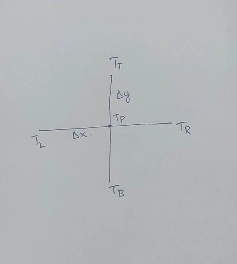
 TL=Left boundary, TT=Top boundary,TP=Point boundary, TR=Right boundary, TB=Bottom boundary

Discretizing the (equation 1)

Tp=(1/k)*(((TL+TR)/dx^2)+((TT+TB)/dy^2))  (equation 2)

 The value of k is k=2((dx^2+dy^2)/(dx^2*dy^2))

Code for the above problem:

Code for jacobi method

clear all
close all
clc
%steady state jacobi iteration
% the boundary of square
L=1;
x=1:10;
dx=abs(x(1)-x(2));
nx=length(x);
y=1:10;
dy=abs(y(1)-y(2));
ny=length(y);
% boundary condtion of square 
t_top = 600;
t_bottom = 900; 
t_Left  = 400;
t_Right = 800;
%initial condtion of first value
t = 400*ones(nx,ny);
t(1,:)=t_top;
t(ny,:)=t_bottom;
t(:,1)=t_Left;
t(:,nx)=t_Right;
t(1,1)=(t_Left+t_bottom)/2;
t(1,ny)=(t_Left+t_top)/2;
t(nx,ny)=(t_top+t_Right)/2;
t(nx,1)=(t_Right+t_bottom)/2;
%assigned initial and old values
t_initial=t;
t_old=t;
% give the tolerance and error
tolerance = 1e-4;
error =1;
%calculation of k value
k=(dx^2*dy^2)/(2*(dx^2+dy^2));
%itration initial value
iteration=1;
% starting the jacobi series loop
while error > tolerance
    %start spatial loops
      for i=2:(length(x)-1)
      for j= 2:(length(y)-1)
          %calculating the temperature jacobi method
          term_1=(t_old((i-1),j)+t_old((i+1),j))/(dx^2);
          term_2=(t_old(i,(j-1))+t_old(i,(j+1)))/(dy^2);
          t(i,j)=k*(term_1+term_2);
          number_of_iteration = num2str(iteration);
      end
      end
      %calculation of error value
      error = max(max(abs(t-t_old)));
      %updating the old value
       t_old=t;
       %updating of iteration
       iteration=iteration+1;
end

%plot the jacobi method
figure(1)
[C,K]=contourf(x,y,t);
clabel(C,K);
colorbar
colormap(jet)
set(gca,'ydir','reverse');
xlabel('x axis')
ylabel('y axis')
title('iteration of jacobi method')

Code explaination

• The input values are assigned. (L,x,dx,nx,y,dy,ny)
• Applying boundary condition of T_top,T_bottom,T_left,T_right.
• Applying initial boundary condition.
• Assigned t_initial=t,t_old=t.
• Given the value of tolerance = 1e-4, error =1
• Finding the k value using this formula k= 2((dx^2+dy^2)/(dx^2*dy^2))
• Applying the initial iteration value = 1
• Now we want to calculate the value of Tp

                     first using convergence loop which is while loop with the condition of error>tolerance

                     Then compute each and every value of i,j. so we use a couple of for loop. 

                      And the Tp value is longer so its is divided into 2 terms After finding those terms addition of that value is calculated Tp.

                     After that spacing values are computated. so end those for loops

• Before that while loop end, we want to updating values of t_old and iteration values error values are calclulated.
• error = max(max(abs(t-t_old)))
• plot of contour function.
• for revercing the value of y in graph using this command set(gca,'ydir','reverse').

Code for gauss seidal method

clear all
close all
clc
%steady state gauss seidal iteration
% the boundary of square
x=1:10;
dx=abs(x(1)-x(2));
nx=length(x);
y=1:10;
dy=abs(y(1)-y(2));
ny=length(y);
% boundary condtion of square 
t_top = 600;
t_bottom = 900; 
t_Left  = 400;
t_Right = 800;
%initial condtion of first value
t = 400*ones(nx,ny);
t(1,:)=t_top;
t(ny,:)=t_bottom;
t(:,1)=t_Left;
t(:,nx)=t_Right;
t(1,1)=(t_Left+t_bottom)/2;
t(1,ny)=(t_Left+t_top)/2;
t(nx,ny)=(t_top+t_Right)/2;
t(nx,1)=(t_Right+t_bottom)/2;
%assigned initial and old values
t_initial=t;
t_old=t;
% give the tolerance and error
tolerance = 1e-4;
error =1;
%calculation of k value
k=(dx^2*dy^2)/(2*(dx^2+dy^2));
%itration initial value
iteration=0;
% starting the gauss seidal loop
while error > tolerance
    %start spatial loops
      for i=2:(length(x)-1)
      for j= 2:(length(y)-1)
          %calculating the temperature gauss seidal method
          term_1=(t((i-1),j)+t_old((i+1),j))/(dx^2);
          term_2=(t(i,(j-1))+t_old(i,(j+1)))/(dy^2);
          t(i,j)=k*(term_1+term_2);
      end
      end
      %calculation of error value
      error = max(max(abs(t-t_old)));
      %updating the old value
       t_old=t;
       %updating of iteration
       iteration=iteration+1;
end
%plot the Gauss seidal method
figure(1)
[c,k]=contourf(x,y,t);
clabel(c,k);
colorbar
colormap(jet)
set(gca,'ydir','reverse');
xlabel('x axis')
ylabel('y axis')
title('Iteration of Gauss seidal method')

Code explaination

• The input values are assigned. (L,x,dx,nx,y,dy,ny)
• Applying boundary condition of T_top,T_bottom,T_left,T_right.
• Applying initial boundary condition.
• Assigned t_initial=t,t_old=t.
• Given the value of tolerance = 1e-4, error =1
• Finding the k value using this formula k= 2((dx^2+dy^2)/(dx^2*dy^2))
• Applying the initial iteration value = 1
• Now we want to calculate the value of Tp

                     first using convergence loop which is while loop with the condition of error>tolerance

                     Then compute each and every value of i,j. so we use a couple of for loop. 

                      And the Tp value is longer so its is divided into 2 terms After finding those terms addition of that value is calculated Tp.

                     After that spacing values are computated. so end those for loops

• Before that while loop end, we want to updating values of t_old and iteration values error values are calclulated.
• error = max(max(abs(t-t_old)))
• plot of contour function.
• for revercing the value of y in graph using this command set(gca,'ydir','reverse').

Coding for SOR method:

clear all
close all
clc
%steady state SOR iteration
% the boundary of square
x=1:10;
dx=abs(x(1)-x(2));
nx=length(x);
y=1:10;
dy=abs(y(1)-y(2));
ny=length(y);
omega=1.2;%thermal diffusivity
% boundary condtion of square 
t_top = 600;
t_bottom = 900; 
t_Left  = 400;
t_Right = 800;
%initial condtion of first value
t = 400*ones(nx,ny);
t(1,:)=t_top;
t(ny,:)=t_bottom;
t(:,1)=t_Left;
t(:,nx)=t_Right;
t(1,1)=(t_Left+t_bottom)/2;
t(1,ny)=(t_Left+t_top)/2;
t(nx,ny)=(t_top+t_Right)/2;
t(nx,1)=(t_Right+t_bottom)/2;
%assigned initial and old values
t_initial=t;
t_old=t;
% give the tolerance and error
tolerance = 1e-4;
error =1;
%calculation of k value
k=(dx^2*dy^2)/(2*(dx^2+dy^2));
%itration initial value
iteration=1;
% starting the SOR series loop
while error > tolerance
    %start spatial loops
      for i=2:(length(x)-1)
      for j=2:(length(y)-1)
          %calculating the temperature jacobi method
          t(i,j)=omega*(0.25*(t(i-1,j)+t_old(i+1,j)+t(i,j-1)+t_old(i,j+1)))+(1-omega)*t_old(i,j);
      end
      end
      %calculation of error value
      error = max(max(abs(t-t_old)));
      %updating the old value
       t_old=t;
       %updating of iteration
       iteration=iteration+1;
end
%plot the sor method
figure(1)
[C,K]=contourf(x,y,t);
clabel(C,K);
colorbar
colormap(jet)
set(gca,'ydir','reverse');
xlabel('x axis')
ylabel('y axis')
title('iteration of SOR method')

Code explaination

• The input values are assigned. (L,x,dx,nx,y,dy,ny,omega)
• Applying boundary condition of T_top,T_bottom,T_left,T_right.
• Applying initial boundary condition.
• Assigned t_initial=t,t_old=t.
• Given the value of tolerance = 1e-4, error =1
• Finding the k value using this formula k= 2((dx^2+dy^2)/(dx^2*dy^2))
• Applying the initial iteration value = 1
• Now we want to calculate the value of Tp

                     first using convergence loop which is while loop with the condition of error>tolerance

                     Then compute each and every value of i,j. so we use a couple of for loop. 

                     After that spacing values are computated. so end those for loops

• Before that while loop end, we want to updating values of t_old and iteration values error values are calclulated.
• error = max(max(abs(t-t_old)))
• plot of contour function.
• for revercing the value of y in graph using this command set(gca,'ydir','reverse').

The 2D heat conduction Transient State general equation is (∂T/∂t)=α((∂^2*T/∂x^2)+(∂^2*T/∂x^2)) 

Discretizing the above equation 

Explicit method

((Tp^(n+1)-Tp^n)/dt) =α*(((Tl-2Tp+Tr)/dx^2)+((Tt-2Tp+Tb)/dy^2))^n (equation 3)

Implicit method

((Tp^(n+1)-Tp^n)/dt) =α*(((Tl-2Tp+Tr)/dx^2)+((Tt-2Tp+Tb)/dy^2))^n+1 (equation 4)

deriving the above (equation 3) (explicit method)

Tp^(n+1)=Tp^n+(k1*(Tl-2Tp+Tr)^n)+(k2*(Tt-2Tp+Tb)

derving the above (equation 4) (implicit method)

Tp^(n+1)= (1/(1+2k1+2k2))*(Tp^n+(k1(Tl+Tr)^n+1)+(k2(Tt+Tb)^n+1))

    where k1=((α*dt)/dx^2)   k2=((α*dt)/dy^2) 

coding for explicit method

clear all
close all
clc
%steady state Explicit iteration
% the boundary of square
x=1:10;
dx=abs(x(1)-x(2));
nx=length(x);
y=1:10;
dy=abs(y(1)-y(2));
ny=length(y);
alpha=1.2; % thermal diffusivity
%defining time step
T=1000;
dt=0.1;
% boundary condtion of square 
t_top = 600;
t_bottom = 900; 
t_Left  = 400;
t_Right = 800;
%initial condtion of first value
t = 500*ones(nx,ny);
t(1,:)=t_top;
t(ny,:)=t_bottom;
t(:,1)=t_Left;
t(:,nx)=t_Right;
t(1,1)=(t_Left+t_bottom)/2;
t(1,ny)=(t_Left+t_top)/2;
t(nx,ny)=(t_top+t_Right)/2;
t(nx,1)=(t_Right+t_bottom)/2;
%assigned initial and old values
t_initial=t;
t_old=t;
%calculation of k value
k_1=alpha*(dt/(dx^2));
k_2=alpha*(dt/(dy^2));
%itration initial value
iteration=0;
% starting the time loop
for k = 1:500
    %start spatial loops
      for i=2:(ny-1)
      for j= 2:(nx-1)
          %calculating the Transient explicit method
          term_1=(t_old(i-1,j)-(2*t_old(i,j))+t_old(i+1,j));
          term_2=(t_old(i,j-1)-(2*t_old(i,j))+t_old(i,j+1));
          t(i,j)=t_old(i,j)+(term_1*k_1)+(term_2*k_2);
          number_of_iteration = num2str(iteration);
      end
      end
      %calculation of error value
      error = max(abs(t_old-t));
      %updating the old value
       t_old=t;
       %updating of iteration
       iteration=iteration+1;
end
%plot the transient explicit method
figure(1)
[C,K]=contourf(x,y,t);
clabel(C,K);
colorbar
colormap(jet)
set(gca,'ydir','reverse');
xlabel('x axis')
ylabel('y axis')
title('Transient explicit method')

Code explaination

• The input values are assigned. (L,x,dx,nx,y,dy,ny,alpha)
• Applying boundary condition of T_top,T_bottom,T_left,T_right.
• Applying initial boundary condition.
• Assigned t_initial=t,t_old=t.
• Given the value of tolerance = 1e-4, error =1
• Finding the k value using this formula k1=((α*dt)/dx^2)   k2=((α*dt)/dy^2) 
• Applying the initial iteration value = 1
• Now we want to calculate the value of Tp

                    There is no need of while loop condition because we don't know only one unknown parameter.

                     Then compute each and every value of i,j. so we use a couple of for loop. 

                      And the Tp value is longer so its is divided into 2 terms After finding those terms addition of that value is calculated Tp.

                     After that spacing values are computated. so end those for loops

• Before that while loop end, we want to updating values of t_old and iteration values error values are calclulated.
• error = max(max(abs(t-t_old)))
• plot of contour function.
• for revercing the value of y in graph using this command set(gca,'ydir','reverse').

Coding for Transient state implicit jacobi method

clear all
close all
clc
%steady state Implicit iteration
% the boundary of square
x=1:10;
dx=abs(x(1)-x(2));
nx=length(x);
y=1:10;
dy=abs(y(1)-y(2));
ny=length(y);
alpha=1.2; % thermal diffusivity
%defining time step
T=1000;
dt=10;
% boundary condtion of square 
t_top = 600;
t_bottom = 900; 
t_Left  = 400;
t_Right = 800;
%initial condtion of first value
t = 500*ones(nx,ny);
t(1,:)=t_top;
t(ny,:)=t_bottom;
t(:,1)=t_Left;
t(:,nx)=t_Right;
t(1,1)=(t_Left+t_bottom)/2;
t(1,ny)=(t_Left+t_top)/2;
t(nx,ny)=(t_top+t_Right)/2;
t(nx,1)=(t_Right+t_bottom)/2;
%assigned initial and old values
t_initial=t;
t_old=t;
%calculation of k value
k_1=alpha*(dt/(dx^2));
k_2=alpha*(dt/(dy^2));
% give the tolerance and error
tolerance = 1e-4;
error =1;
%itration initial value
iteration=0;
%starting the time loop
for nt=1:1500
    % starting the Implicit jacobi series loop
while error > tolerance
    %start spatial loops
      for i=2:(ny-1)
      for j= 2:(nx-1)
          %calculating the temperature Transient state jacobi method
          term_1=1/(1+(2*k_1)+(2*k_2));
          term_2=k_1*term_1;
          term_3=k_2*term_1;
          h=(t_old(i-1,j)+t_old(i+1,j));
          v=(t_old(i,j-1)+t_old(i,j+1));
          t(i,j)=(t_initial(i,j)*term_1)+(h*term_2)+(v*term_3);
          number_of_iteration = num2str(iteration);
      end
      end
      %calculation of error value
      error = max(max(abs(t-t_old)));
      %updating the old value
       t_old=t;
       %updating of iteration
       iteration=iteration+1;
end
% updating t initial value
t_initial = t;
end
%plot the Transient state jacobi method
figure(1)
[C,K]=contourf(x,y,t);
clabel(C,K);
colorbar
colormap(jet)
set(gca,'ydir','reverse');
xlabel('x axis')
ylabel('y axis')
title('Transient state Implicit jacobi method')

Code explaination

• The input values are assigned. (L,x,dx,nx,y,dy,ny,alpha)
• Applying boundary condition of T_top,T_bottom,T_left,T_right.
• Applying initial boundary condition.
• Assigned t_initial=t,t_old=t.
• Given the value of tolerance = 1e-4, error =1
• Finding the k value using this formula k1=((α*dt)/dx^2)   k2=((α*dt)/dy^2)
• Applying the initial iteration value = 1
• Now we want to calculate the value of Tp

                     first using convergence loop which is while loop with the condition of error>tolerance

                     Then compute each and every value of i,j. so we use a couple of for loop. 

                      And the Tp value is longer so its is divided into 2 terms, H and V After finding those terms addition of that value is calculated Tp.

                     After that spacing values are computated. so end those for loops

• Before that while loop end, we want to updating values of t_old and iteration values error values are calclulated.
• error = max(max(abs(t-t_old)))
• plot of contour function.
• for revercing the value of y in graph using this command set(gca,'ydir','reverse').

Code for Transient state gauss seidal method

clear all
close all
clc
%steady state Implicit iteration
% the boundary of square
x=1:10;
dx=abs(x(1)-x(2));
nx=length(x);
y=1:10;
dy=abs(y(1)-y(2));
ny=length(y);
alpha=1.2; % thermal diffusivity
%defining time step
T=1000;
dt=10;
% boundary condtion of square 
t_top = 600;
t_bottom = 900; 
t_Left  = 400;
t_Right = 800;
%initial condtion of first value
t = 500*ones(nx,ny);
t(1,:)=t_top;
t(ny,:)=t_bottom;
t(:,1)=t_Left;
t(:,nx)=t_Right;
t(1,1)=(t_Left+t_bottom)/2;
t(1,ny)=(t_Left+t_top)/2;
t(nx,ny)=(t_top+t_Right)/2;
t(nx,1)=(t_Right+t_bottom)/2;
%assigned initial and old values
t_initial=t;
t_old=t;
%calculation of k value
k_1=alpha*(dt/(dx^2));
k_2=alpha*(dt/(dy^2));
% give the tolerance and error
tolerance = 1e-4;
error =1;
%itration initial value
iteration=0;
%starting the time loop
for nt=1:1500
    % starting the Implicit Gauss seidal loop
while error > tolerance
    %start spatial loops
      for i=2:(ny-1)
      for j= 2:(nx-1)
          %calculating the temperature Transient state Gauss seidal method
          term_1=1/(1+(2*k_1)+(2*k_2));
          term_2=k_1*term_1;
          term_3=k_2*term_1;
          h=(t(i-1,j)+t_old(i+1,j));
          v=(t(i,j-1)+t_old(i,j+1));
          t(i,j)=(t_initial(i,j)*term_1)+(h*term_2)+(v*term_3);
          number_of_iteration = num2str(iteration);
      end
      end
      %calculation of error value
      error = max(max(abs(t-t_old)));
      %updating the old value
       t_old=t;
       %updating of iteration
       iteration=iteration+1;
end
% updating t initial value
t_initial = t;
end
%plot the Transient state Gauss seidal method
figure(1)
[C,K]=contourf(x,y,t);
clabel(C,K);
colorbar
colormap(jet)
set(gca,'ydir','reverse');
xlabel('x axis')
ylabel('y axis')
title('Transient state Implicit Guass seidal method')

Code explaination

• The input values are assigned. (L,x,dx,nx,y,dy,ny,alpha)
• Applying boundary condition of T_top,T_bottom,T_left,T_right.
• Applying initial boundary condition.
• Assigned t_initial=t,t_old=t.
• Given the value of tolerance = 1e-4, error =1
• Finding the k value using this formula k1=((α*dt)/dx^2)   k2=((α*dt)/dy^2)
• Applying the initial iteration value = 1
• Now we want to calculate the value of Tp

                     first using convergence loop which is while loop with the condition of error>tolerance

                     Then compute each and every value of i,j. so we use a couple of for loop. 

                      And the Tp value is longer so its is divided into 2 terms, H and V After finding those terms addition of that value is calculated Tp.

                     After that spacing values are computated. so end those for loops

• Before that while loop end, we want to updating values of t_old and iteration values error values are calclulated.
• error = max(max(abs(t-t_old)))
• plot of contour function.
• for revercing the value of y in graph using this command set(gca,'ydir','reverse').

Code for Transient state SOR method

clear all
close all
clc
%steady state SOR iteration
% the boundary of square
x=1:10;
dx=abs(x(1)-x(2));
nx=length(x);
y=1:10;
dy=abs(y(1)-y(2));
ny=length(y);
omega=1.2;%thermal diffusivity
% boundary condtion of square 
t_top = 600;
t_bottom = 900; 
t_Left  = 400;
t_Right = 800;
%initial condtion of first value
t = 400*ones(nx,ny);
t(1,:)=t_top;
t(ny,:)=t_bottom;
t(:,1)=t_Left;
t(:,nx)=t_Right;
t(1,1)=(t_Left+t_bottom)/2;
t(1,ny)=(t_Left+t_top)/2;
t(nx,ny)=(t_top+t_Right)/2;
t(nx,1)=(t_Right+t_bottom)/2;
%assigned initial and old values
t_initial=t;
t_old=t;
% give the tolerance and error
tolerance = 1e-4;
error =1;
%calculation of k value
k=(dx^2*dy^2)/(2*(dx^2+dy^2));
%itration initial value
iteration=1;
% starting the jacobi series loop
while error > tolerance
    %start spatial loops
      for i=2:(nx-1)
      for j= 2:(ny-1)
          %calculating the temperature jacobi method
         t(i,j)=omega*(0.25*(t(i-1,j)+t_old(i+1,j)+t(i,j-1)+t_old(i,j+1)))+(1-omega)*t_old(i,j);
      end
      end
      %calculation of error value
      error = max(max(abs(t-t_old)));
      %updating the old value
       t_old=t;
       %updating of iteration
       iteration=iteration+1;
end
%plot the sor method
figure(1)
[C,K]=contourf(x,y,t);
clabel(C,K);
colorbar
colormap(jet)
set(gca,'ydir','reverse');
xlabel('x axis')
ylabel('y axis')
title('iteration of SOR method')

• The input values are assigned. (L,x,dx,nx,y,dy,ny,alpha)
• Applying boundary condition of T_top,T_bottom,T_left,T_right.
• Applying initial boundary condition.
• Assigned t_initial=t,t_old=t.
• Given the value of tolerance = 1e-4, error =1
• Finding the k value using this formula k1=((α*dt)/dx^2)   k2=((α*dt)/dy^2)
• Applying the initial iteration value = 1
• Now we want to calculate the value of Tp

                     first using convergence loop which is while loop with the condition of error>tolerance

                     Then compute each and every value of i,j. so we use a couple of for loop. 

                     After that spacing values are computated. so end those for loops

• Before that while loop end, we want to updating values of t_old and iteration values error values are calclulated.
• error = max(max(abs(t-t_old)))
• plot of contour function.
• for revercing the value of y in graph using this command set(gca,'ydir','reverse').

Conclusion

     i) Jacobi>Gauss seidal>SOR number of iteration all methods scheme.

    ii) steady state is successful and takes least time to computate.

    iii) SOR method is effective iteration method.