Week 9 - FVM Literature Review

Objective

1. Finite Volume Method(FVM)

2.The major differences between FDM & FVM

3.The need for interpolation schemes and flux limiters in FVM

4.use the 1D linear heat conduction equation

1.Finite Volume Method

The finite volume method(FVM) is a discretization technique for partial differential equation,especially those that arise from physical conservation laws.FVM uses a volume intergral formulation of the problem with the finite partitioning set of volumes to discretize the equation.FVM is in common use for discretizing computational fluid dynamics equations.

2.Difference between Finite difference and Finite volume Methods

FINITE DIFFERENCE METHOD	FINITE VOLUME METHOD
1.Uses regular grid	1.Can use irregular grid
2.Incremental time steps need to be smaller than critical value for stability	2.Time steps can be larger with unconditionally stable schemes
3.Small amount of calculations in each time step	3.Large amount of calculations in each time step
4.No iteration necessary to follow nonlinear consitutive law	4.To follow a nonlinear consitutive law an iterative procedure is required
5.Following nonlinear laws in a valid physical way is guaranted	5.The following of physically correct path should always be assured
6.Low memory requirement for storage of stiffness matrices	6.Large memory requirement for storage of stiffness matrices

3.Need of Interpolation scheme and flux limiter in FVM

interpolation and Need of interpolation

Need of interpolation.

Interpolation is needed to compute the value of a function for an intermediate value of the independent function.

Interpolation

Interpolation schemes are used to transform cell-centre quantities to face centres. The operation is used in many of the finite volume calculations, e.g. for the calculation of gradient, divergence, and Laplacian terms.

Types of interpolation

• Upwind interpolation.
• Linear interpolation(CDS).
• Quadratic upwind interpolation(QUICK) and etc.

Upwind interpolation.

In computational physics, the term upwind scheme typically refers to a class of numerical discretization methods for solving hyperbolic partial differential equations, in which so-called upstream variables are used to calculate the derivatives in a flow field.

Linear interpolation(CDS).

Central differences are useful in solving partial differential equations. If the data values are available both in the past and in the future, the numerical derivative should be approximated by the central difference.

Quadratic upwind interpolation(QUICK).

In computational physics, the term upwind scheme typically refers to a class of numerical discretization methods for solving hyperbolic partial differential equations, in which so-called upstream variables are used to calculate the derivatives in a flow field.

Flux limiter in interpolation

1 These are used in high resolution schemes.these help in limtting the resolution gradient near shocks and discontinunities.Objective of implementing flux limiter schemes is to control the spartial derivatives the realistic values.

2.The limiter function is greater than or equal to zero,i.e when the limiter is equal to zero than the flux is represented by low resolution schemes.

3.Flux limiter also called slope limiter as they have some mathematical form and they can help in limiting the solution grandient near shocks and discountinunties.

4.The flux limitter is used when the limitter acts on the system fluxes and slope limitter is used when the limitter acts on the system(like pressure and velocity).

5.This factor are selected as per the given problem and the scheme used for the solution.

4. 1D linear heat conduction equation

1.Once we have this intergral form of equation

2.Apply Gauss divergence theorem

3.We get descretized form which can be solved using computer ("flux term").

A staedy state heat conduction equation with heat gradient - ∂/∂x(α.(∂T/∂x)) + S = 0

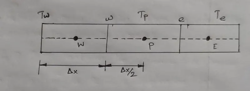
S is source term, α is Thermal diffusivity term, (∂T/∂x) is is temperature gradient along with x axis.

Governing equation - ∂/∂x(α.(∂T/∂x)) + S = 0 is valid at every point in domain, which means it is also valid in entire control volume.

if small control volume (dv) is considered and it is multiplied with the governing equation and intergrated it for entire volume than that should be also equal to zero is the Intergral foam of governing equation.

Multiplying the equation by 'dv' and integrating it

∫(∂/∂x(α.(∂T/∂x)) + S)dv = 0

∫∂/∂x(α.(∂T/∂x))dv + ∫Sdv =0

if dv = A.dx

∫∂/∂x(α.(∂T/∂x)) A.dx +∫S A.dx = 0

[ αA.(∂T/∂x)]upper limit e, lower limit ω + s¯dv = 0

s¯ is average value of source term (S) which when multiply by dv is going to be equal to ∫Sdv

αeA.(∂T/∂xe)-αωA.(∂T/∂xω)+s¯dv = 0

If we assume α is constant

αA.[(Te-Tp)/△x]-αA.[(Te-Tp)/△x]+s¯dv = 0

The source term which is to be added cell, α is a function of temperature

(s¯linearization -- Su+SpTp)

αA.[(Te-Tp)/△x]-αA.[(Te-Tp)/△x]+s¯dv = 0

[Heat flux]out - [Heat flux]in + sourceterm = 0

The amount of heat that is removed from perticular box is conserved.