Week 5 - Rayleigh Taylor Instability

Aim

Simulate Rayleigh Taylor instability

Objectives

1. What are some practical CFD models that have been based on the mathematical analysis of Rayleigh Taylor waves? In your own words, explain how these mathematical models have been adapted for CFD calculations.
2. Perform the Rayleigh Taylor instability simulation for 2 different mesh sizes with the base mesh being 0.5 mm. Compare the results by showing the animations (Attach them from your google drive). Observe the differences in the animation and explain the effect of mesh size on simulation. Also, explain why a steady-state approach might not be suitable for these types of simulation.[ Choose Air and Water for this simulation]
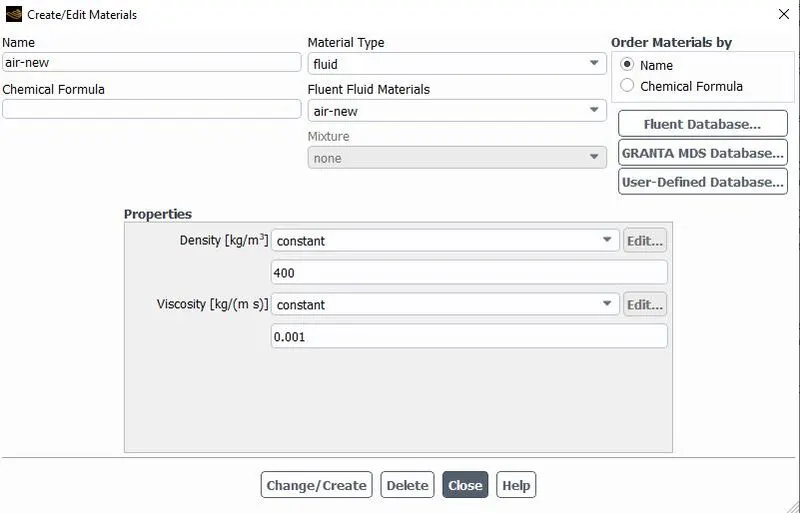
3. Run one more simulation with water and user-defined material (density = 400 kg/m³, viscosity = 0.001 kg/m-s) for refined mesh.
4. Define the Atwood Number. Find out the Atwood number for both the cases and explain how the variation in Atwood number in the above two cases affects the behavior of the instability

Methodology

• Introduction

Rayleigh Taylor instability is instability at the interface when two fluids of different density contacts each other. In this scenario, the lighter fluid pushes the heavier fluid in the gravitational field.

Following are some practical CFD models that have been used in the mathematical analysis of Rayleigh Taylor waves.

• Plateau-Rayleigh instability

This is often called Rayleigh instability. It explains why and how a falling stream of fluid breaks up into smaller packets with the same volume but less surface area. It is related to the Rayleigh–Taylor instability and is part of a greater branch of fluid dynamics concerned with fluid thread breakup. This fluid instability is exploited in the design of a particular type of inkjet technology whereby a jet of liquid is perturbed into a steady stream of droplets.

• Kelvin–Helmholtz instability

The Kelvin–Helmholtz instability (after Lord Kelvin and Hermann von Helmholtz) is a fluid instability that occurs when there is velocity shear in a single continuous fluid or a velocity difference across the interface between two fluids.

• Richtmyer–Meshkov instability

It occurs when two fluids of different densities are impulsively accelerated. Normally this is by the passage of a shock wave. The development of the instability begins with small amplitude perturbations which initially grow linearly with time. This is followed by a nonlinear regime with bubbles appearing in the case of a light fluid penetrating a heavy fluid, and with spikes appearing in the case of a heavy fluid penetrating a light fluid

1. Preprocessing

• Model creation

In this Rayleigh Taylor instability problem, we will be modeling a 2D geometry that represents two fluids. One is air and one is Water. The less-dense water is considered at the bottom and water is considered on the top.

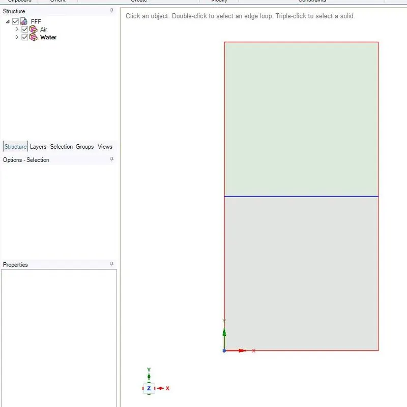
A geometry of 20x40mm is taken in which lower 20x20mm is air and upper 20x20mm is water.

The above said geometry is created in Ansys Spaceclaim. After creating the geometry, go to the workbench and share the interface in order to make a conformal meshing.

• Meshing

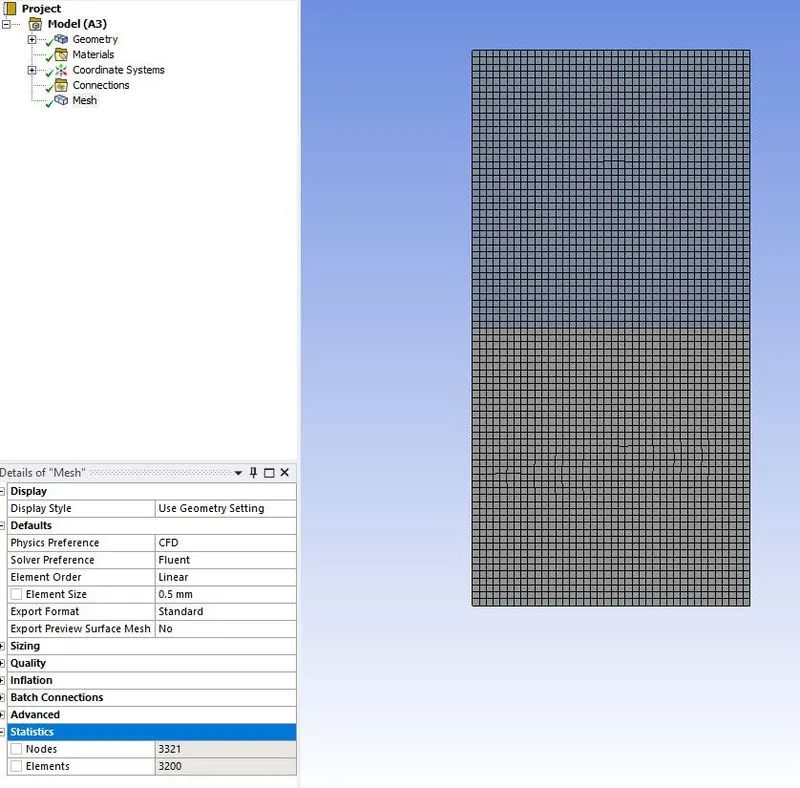
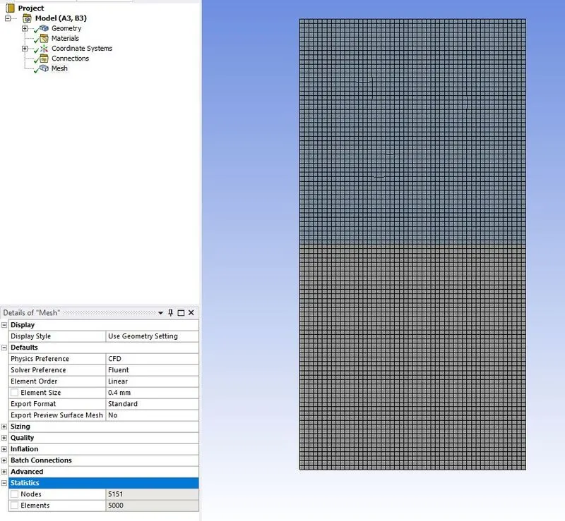
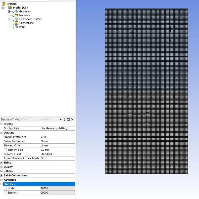
Since our geometry is simple 2D, we will be doing simple meshing. Open the mesh window. Click on mesh, on the properties, change the element size to 0.5mm. Then click on generate mesh and update. Similarly, we will be doing element sizes of 0.4mm and 0.3mm.

The generated mesh will look as follows,

Element size = 0.5mm

Element size = 0.4mm

Element size = 0.3mm

• Setting up the problem

Here we set up the problem by applying relevant

• Initial conditions
• Boundary conditions
• Material properties
• Turbulence Models

As we simulate Rayleigh Taylor instability, we are interested to see how the interface between the two phases collapses as the function of time, transient simulation is used. We also need gravity enabled. Since it is a 2d geometry gravity will be acting in the y axis.

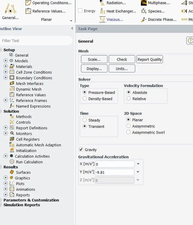
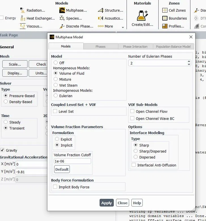
Next is setting up the physics, there is no need for energy and we will be considering Laminar flow. Since two-fluid interaction is involved, multiphase need to be turned on. In the multiphase window enable Volume of Fluid model, in which we will be modeling 2 Eulerian Phases. We will be doing an implicit formulation as this formulation is highly stable and requires lesser time compared to the explicit formulation.

Material Properties

We have two materials, one is Air and the second is Water. Also, we will be doing a simulation using user-defined material.

Air Properties

Density = `1.225 (kg)/m^3`

Kinematic viscosity = `1.7894*10^5 (kg)/(ms)`

Water properties

Density = `998.2 (kg)/m^3`

Kinematic viscosity = `0.001003 (kg)/(ms)`

User Material

Density =`400 (kg)/m^3`

Kinematic viscosity =`0.001 (kg)/(ms)`

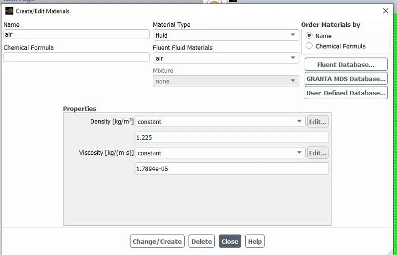
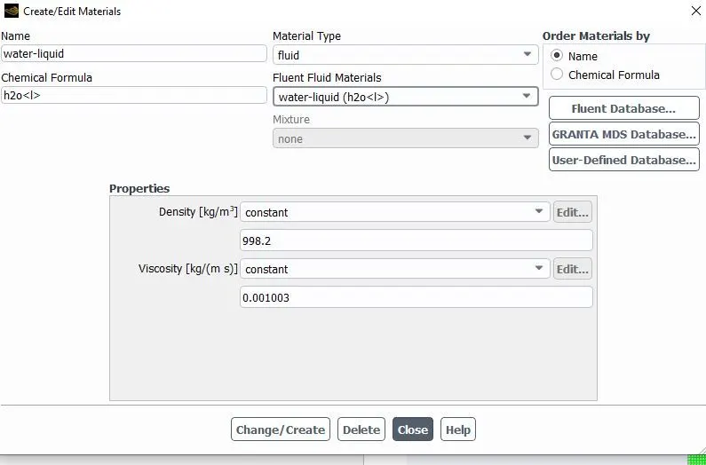
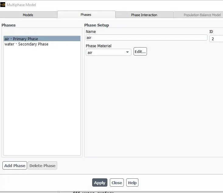
The next step is to label the different phases. For that, click on multiphase then go to phases. Rename Primary Phase to air and select Air as phase material. Rename Secondary Phase to water and select water as phase material. Click on apply and close the window.

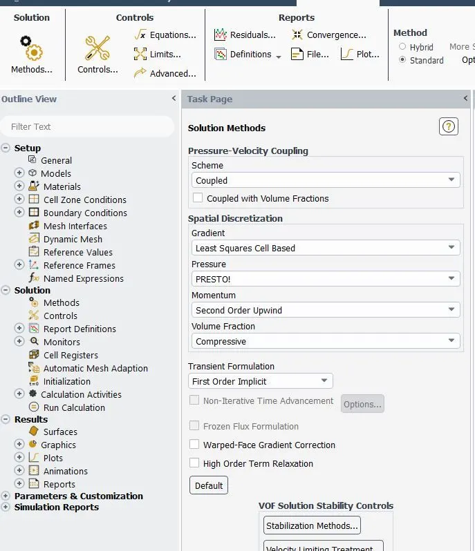
Let’s select the solution method as coupled and choose hybrid initialization and initialize the solution.

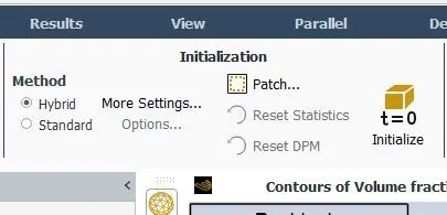
After initialization, an option called patch will be visible on the initialization tab. Since this is a multiphase problem, we need to tell the solver that in which surface the water or Air is situated. For that click on Patch, then select water as phase, click on volume fraction. At the zones to patch click on the water surface and give value 1. Then click on patch. Then deselect the water surface under zones and select air surface and put value 0 and click on patch.

Here the value 1 represents present, and value 0 represents absent. So here we are trying to tell the solver that the water is present at the zone named water_suface and water is absent at the zone named air_surface.

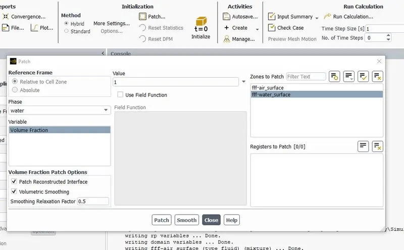
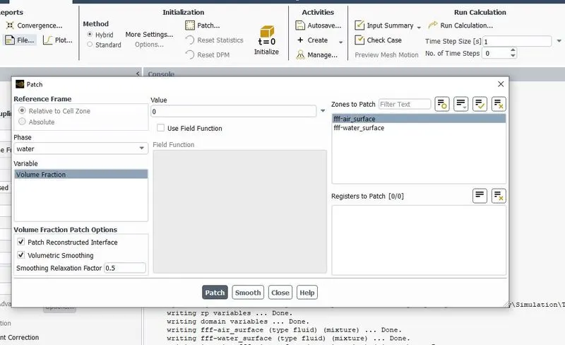
To check whether the above process is completed successfully, insert a contour plot of phases. For that, go to the Results tab, click on contours, and create new, select phases as contour and water as the phase. After this, select all the surfaces then click on compute and click on save and display.

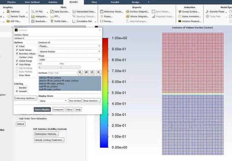
From the above contour, we can understand the above surface (reddish) is filled with water and the bottom surface is air as the water fraction is zero (blue).

To study how the instability is progressing over time during the simulation, the animation is also created.

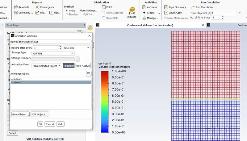
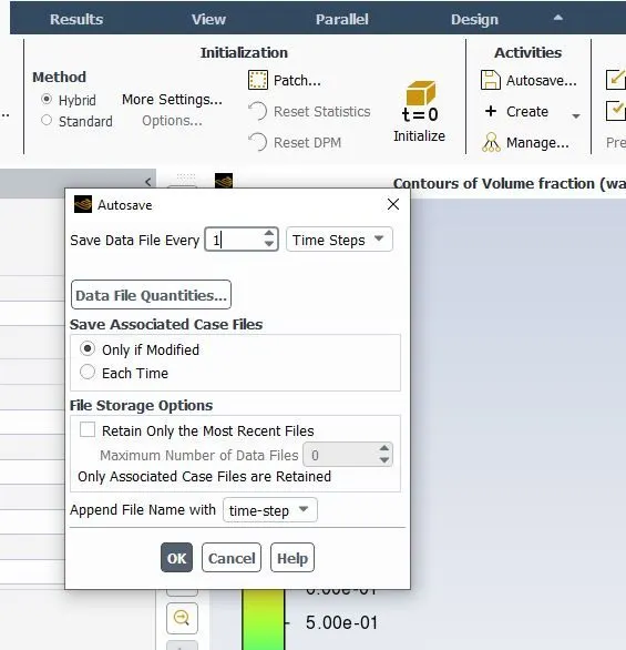
The autosave option is turned on in order to replicate the results in the CFD post.

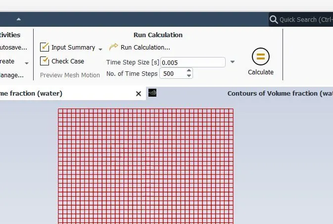
After doing all the above-mentioned setups, the solver is ran 500-time steps with a step size of 0.005 seconds. So a total of 2.5s.

1. Postprocessing
   1. Solutions: Water and Air

Water properties

Density = `998.2 (kg)/m^3`

Kinematic viscosity = `0.001003 (kg)/(ms)`

Air Properties

Density = `1.225 (kg)/m^3`

Kinematic viscosity = `1.7894*10^5 (kg)/(ms)`

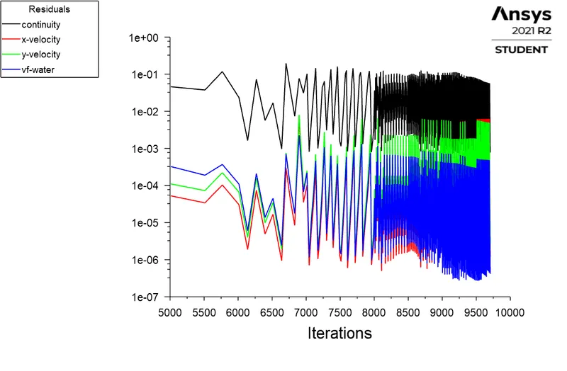
• Residual plot
  • Element size 0.5mm
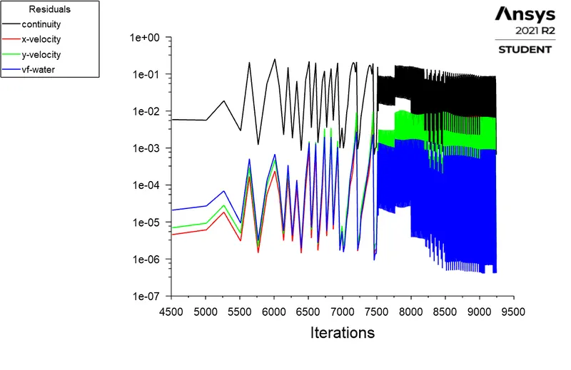
  • Element Size = 0.4mm
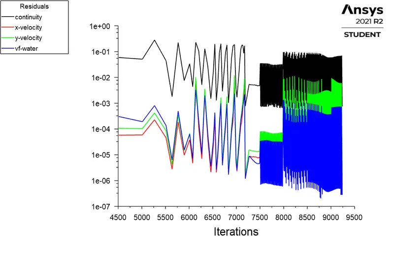
  • Element Size = 0.3mm
• Phase contour at 15-time step

Element size = 0.5mm

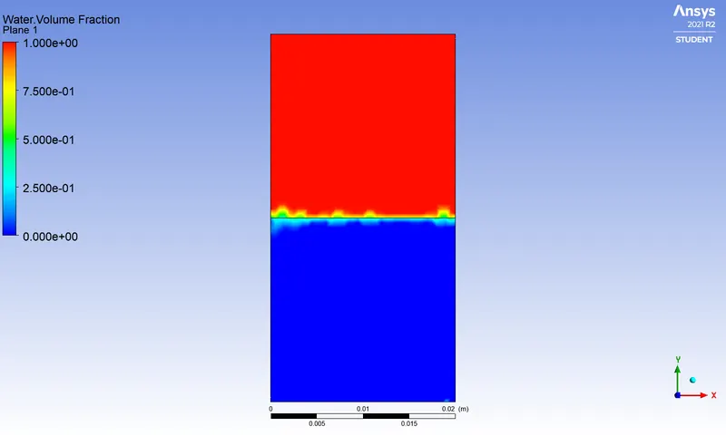
Element Size = 0.4mm

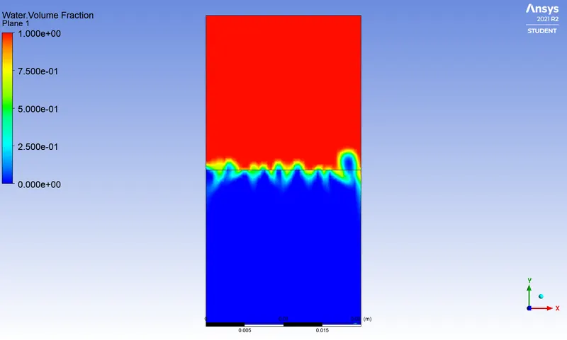
Element size = 0.3mm

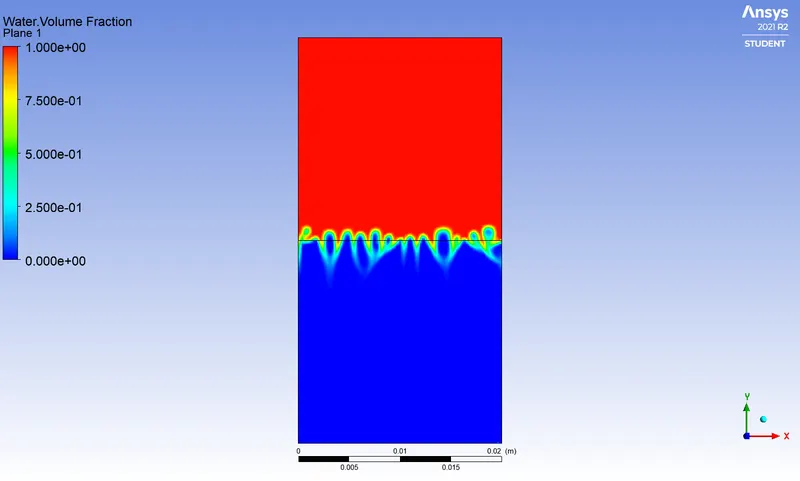
• Phase contour at 250-time step

Element size = 0.5mm

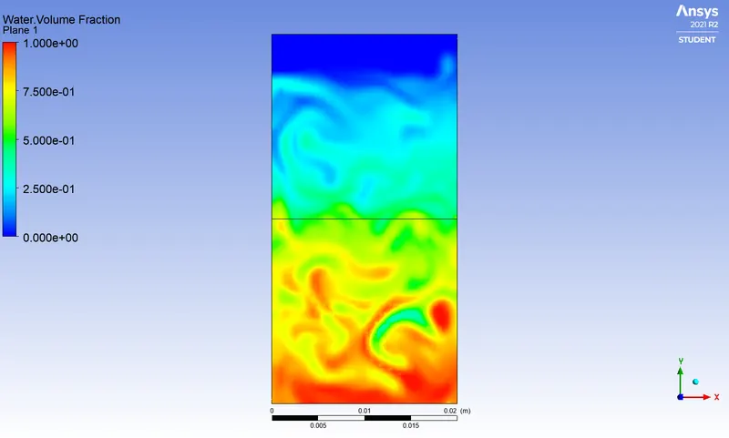
Element Size = 0.4mm

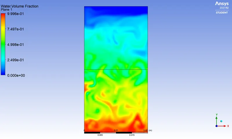
Element Size = 0.3mm

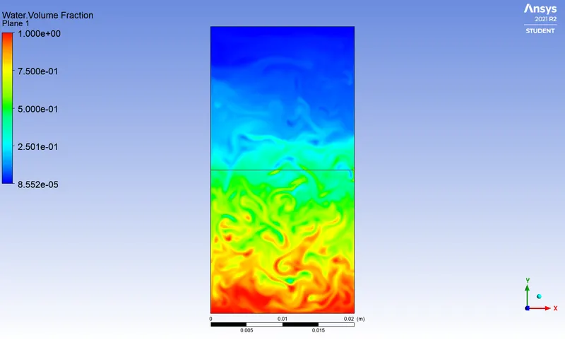
• Phase contour at 500-time step

Element size = 0.5mm

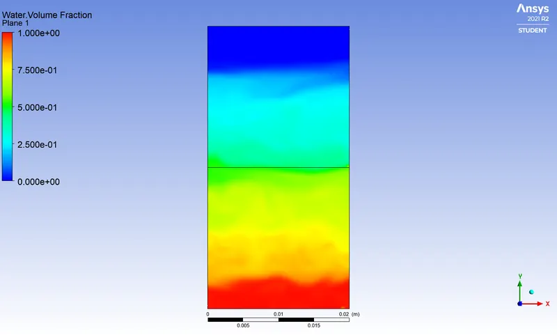
Element size = 0.4mm

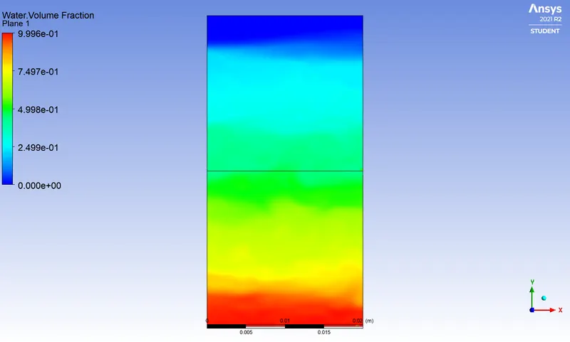
Element size = 0.3mm

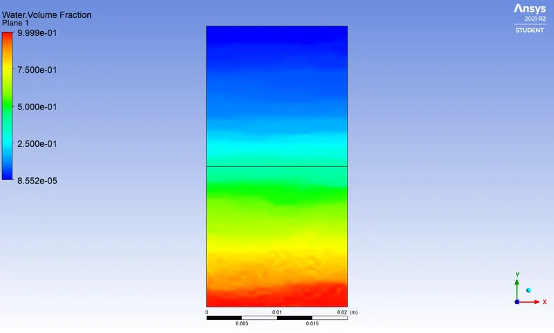
The above plots show the behavior of the two phases with different refinement and at different time steps. It is observed that at a particular time step the refined mesh captures more physics than the other two mesh sizes. For example, after 15 time steps the mesh with 0.3mm element size gives a clear and detailed instability between the two phases than 04mm and 0.5mm element sizes. After completing a 500-time step, we can see the refined mesh shows a clear water region at the bottom.

An animated video is attached hereto visualize the flow over time.

1. Element size 0.5mm

https://drive.google.com/file/d/1mrmP4PvEsFfX4FB8JnhsGfzxEMaTZANe/view?usp=sharing

2. Element size=0.4mm

https://drive.google.com/file/d/1YD3H1YWvAF01j6tRn9tXPVx4PNE1WRgK/view?usp=sharing

3.Element size = 0.3mm

https://drive.google.com/file/d/1URmrNrsN3a-2M3incAigPJjy3droTECJ/view?usp=sharing

2. Solution: Water and User material

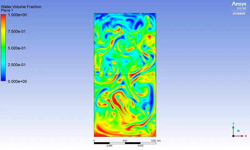
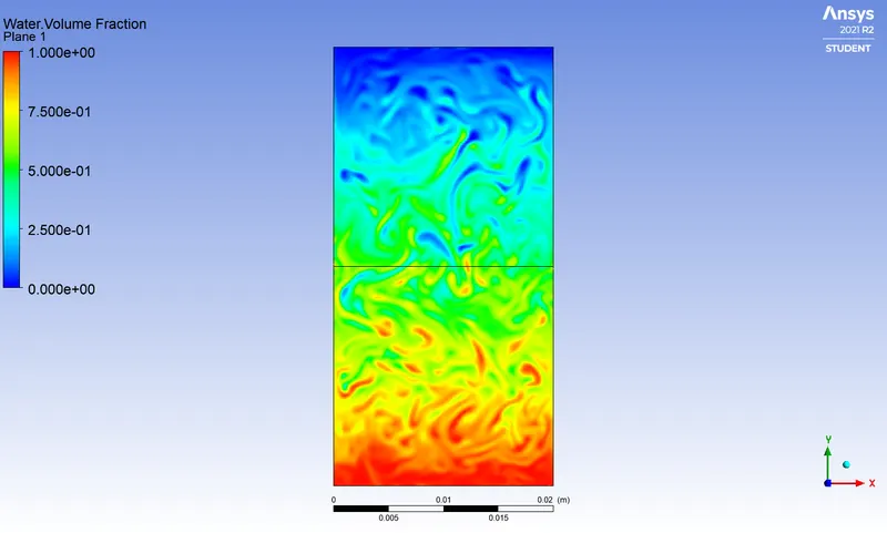
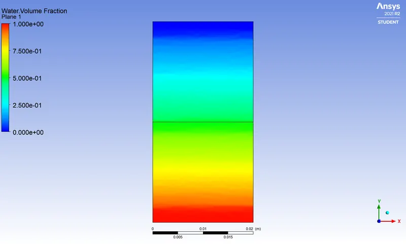
The following results are obtained by using water and custom material. We had to run for 1500 time steps (7.5s) keeping a step size of 0.005s in order to get a realizable result.

Water properties

Density = `998.2 (kg)/m^3`

Kinematic viscosity = `0.001003 (kg)/(ms)`

User Material

Density =`400 (kg)/m^3`

Kinematic viscosity =`0.001 (kg)/(ms)`

• Residual Plot.

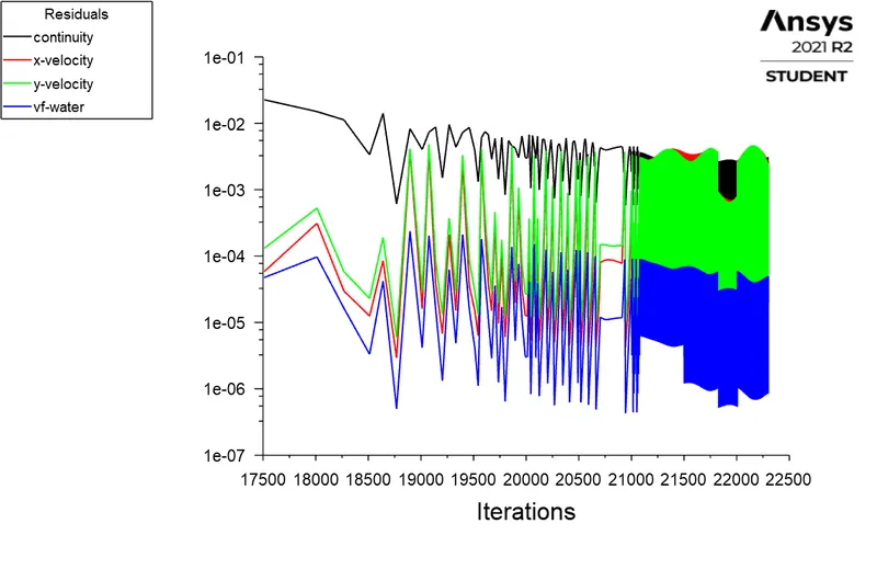
• Phase contour at different time steps
  • 50-time steps
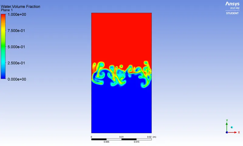
  • 250-time steps
  • 500-time steps
  • 
  • 1500-time steps

The above plots show the contour plots when one phase is user material and one phase is water. It shows that it needs more time to settle down the instability compared to the air-water case. The reason behind this is that the user material has more density than the air.

An animate video is attached here

https://drive.google.com/file/d/1-BV36aL_ZqzfkpXMfRtN00GlGbwnyAOz/view?usp=sharing

Atwood number

Atwood number (A) is a dimensionless density ratio that is used in fluid dynamics to study the hydrodynamic instabilities in density stratified flows. It is defined as,

`A= (ρ_1-ρ_2)/(ρ_1+ρ_2 )`

Where,

`ρ_1=` density of the heavier fluid

`ρ_2=` density of the lighter fluid

Case 1: Air and water

`ρ_1=998.2`

`ρ_2=1.225`

`A= (998.2-1.225)/(998.2+1.225)=0.9975`

Case 2: User material and Water

`ρ_1=998.2`

`ρ_2=400`

`A= (998.2-400)/(998.2+400)=0.428`

In Rayleigh–Taylor instability, the penetration distance of heavy fluid bubbles into the lighter fluid is a function of the acceleration time scale, `A*g*t^2` where g is the gravitational acceleration and t is the time.

In case 1, A is close to 1, hence penetration distance is more therefore penetration happens very fast.

In case 2, A is very less, hence penetration distance is less therefore penetration happens very slowly.

Conclusions

1. From the studies conducted above, we can observe that as the mesh becomes finer the instabilities are captured better. But ad it becomes finer the computational time is also getting more.
2. Since we are studying the instabilities and these are unpredictably varying as a function of time, steady-state simulation cannot capture this phenomenon. Hence transient simulation is preferred.
3. Atwood number is helpful in predicting the instability of the interface with help of a dimensionless parameter as we saw above.